Rainfall-runoff Modelling in a Semi-urbanized Catchment using

Self-adaptive Fuzzy Inference Network

Tak Kwin Chang

, Amin Talei

and Chai Quek

School of Engineering, Monash University Malaysia, Jalan Lagoon Selatan,

Bandar Sunway, 47500 Subang Jaya, Malaysia

Center for Computational Intelligence, Nanyang Technological University, School of Computer Engineering,

50, Nanyang Avenue, Singapore 639798, Singapore

Keywords: Rainfall-runoff Modelling, Neuro-fuzzy Systems, SaFIN, ANFIS, SWMM, ARX.

Abstract: Conventional neuro-fuzzy systems used for rainfall-runoff (R-R) modelling generally employ offline learning

in which the number of rules and rule parameters need to be set by the user in calibration stage. This make

the rule-base fixed and incapable of being adaptive if some rules become inconsistent over time. In this study,

the Self-adaptive Fuzzy Inference Network (SaFIN) is used for R-R application. SaFIN benefits from an

adaptive learning mechanism which allows it to remove inconsistent and obsolete rules over time. SaFIN

models are developed to capture the R-R process in two catchments including Dandenong located in Victoria,

Australia, and Sungai Kayu Ara catchment in Selangor, Malaysia. Models’ performance aer then compared

with the ANFIS, ARX, and physical models. Results show that SaFIN outperforms ANFIS, ARX, and

physical models in simulating runoff for both low and peak flows. This study shows the good potential of

using SaFIN in R-R modelling application.

1 INTRODUCTION

Rainfall-runoff (R-R) modelling as one of the

important topics in hydrology is focused on better

understanding of the rainfall-runoff process which is

necessary to address some of hydrological problems

such as urban water management and flood

forecasting. In addition to physical and conceptual

models, there is a third group of R-R models known

as system theoretic models which involves a direct

mapping (linear/non-linear) between the inputs and

output data (Minns and Hall, 1996). System theoretic

models do not use the knowledge of the system’s

parameters directly but instead formulate its own set

of parameters based purely on the dataset. Examples

of such models are regression-based models,

Artificial Neural Networks (ANN), and Neuro-Fuzzy

Systems (NFS) (Xiong et al., 2001, Rajurkar et al.,

2002, Sajikumar and Thandaveswara, 1999). NFS are

hybridizations of fuzzy set theory and neural

networks which provide the mapping of input-output

data with varying degrees of non-linearity. NFS

learning can generally be classified as either offline

learning or online learning systems. Offline or batch

learning formulates model parameters based on a

static dataset, whereas online learning enables models

to sequentially update its parameters during each

timestep of the training data. The benefit of online

learning models is that it allows a model to inherit a

dynamic training approach where the model

parameters evolves sequentially as new data becomes

available, enabling the model to capture time varying

properties within the system; whereas offline learning

models requires a retraining process of the entire

dataset merged with new data to achieve similar

results, resulting in greater computational time and

complexity.

NFS models with offline learning such as

Adaptive Network-based Fuzzy Inference System

(ANFIS) are extensively used in R-R modelling

(Nayak et al., 2004, Nayak et al., 2005, Remesan et

al., 2009, Mukerji et al., 2009, Talei et al., 2010b,

Talei et al., 2010a, Bartoletti et al., 2017, Zakhrouf et

al., 2015). The major drawback of a model such as

ANFIS is its offline learning algorithm where the

number of rules is pre-set by the user and remains

fixed. In real-world applications, a reliable R-R

model should be able to dynamically capture time-

varying properties within a system through a

continuous process of updating and reiterating its

Chang, T., Talei, A. and Quek, C.

Rainfall-runoff Modelling in a Semi-urbanized Catchment using Self-adaptive Fuzzy Inference Network.

DOI: 10.5220/0007227300860097

In Proceedings of the 10th International Joint Conference on Computational Intelligence (IJCCI 2018), pages 86-97

ISBN: 978-989-758-327-8

model parameters. To date, not many studies have

been made on addressing adaptability through online

learning adaptation in R-R modelling. In recent

literature, several authors have attempted

incorporating online learning into various R-R

modelling applications and has generally shown

improvement in modelling performance (Hong, 2012,

Luna et al., 2007, Talei et al., 2013, Ashrafi et al.,

2017, Chang et al., 2016). In this study, Self-adaptive

Fuzzy Inference Network (SaFIN) (Tung et al., 2011)

is adopted and applied in developing a R-R model.

SaFIN is known for its capability of being self-

adaptive which enable the learning mechanism to add

and remove rules automatically. This study aims to

investigate the capabilities of using SaFIN as a R-R

model while comparing its performance with ANFIS

and a physical benchmark model known as Storm

Water Management Model (SWMM).

2 SELF-ADAPTIVE FUZZY

INFERENCE NETWORK

(SaFIN)

SaFIN is a self-organizing neural fuzzy system with

incremental online learning capabilities developed by

Tung et al (2011). SaFIN is a fully data-driven model

capable of formulating and maintaining a consistent

rule-base automatically. SaFIN was developed to

address several issues faced in previously existing

models such as inconsistencies within the rulebase,

the need for prior knowledge, and addressing the

stability-plasticity tradeoff. SaFIN consists of a five-

layer multilayer perceptron (MLP) network which

employs the neural network-based gradient descent

approach to fine-tune the parameters of its

membership functions. In conventional neuro-fuzzy

systems, the fuzzy clusters and fuzzy rule base require

initialization through the knowledge of human

experts. To address this issue, SaFIN employs two

learning mechanisms: (1) self-organizing clustering,

and (2) self-automated rule generation (Tung et al,

2011). Through the self-organizing clustering

technique, the numbers, positions, and spreads of

fuzzy labels are self-determined from the training

dataset. This clustering technique of SaFIN is known

as Categorical-Learning Induced Partitioning (CLIP).

The main motivation for using CLIP is the fact that it

is a tailored approach for addressing the stability-

plasticity dilemma of NFS models. CLIP draws

inspiration from the behavioural category learning

process exhibited by humans whereby categorical

learning builds up from a basic high-contrasting level

of distinction to a low-contrasting categorical

distinction. CLIP represents these categorical

distinctions as Gaussian membership functions where

the parameters α and β allows direct control of these

fuzzy labels. Membership functions transfer the crisp

values of input space to fuzzy values. Although there

are several mathematical functions that can be used

for this purpose, Tung et al (2011) suggested using

Gaussian membership function in CLIP.

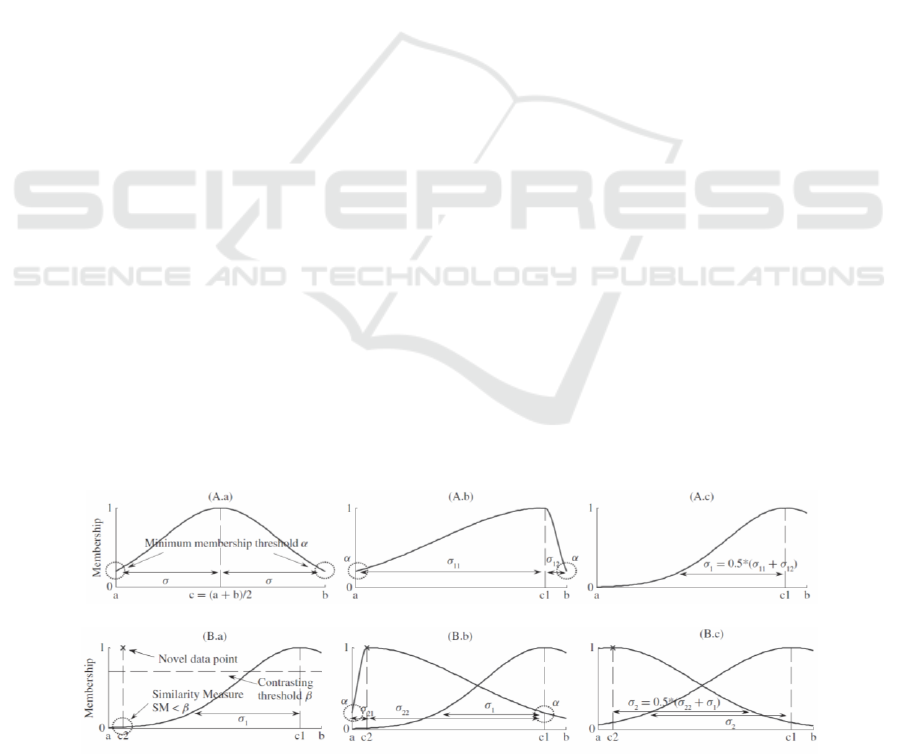
Figure 1 shows the fuzzy partitioning process of CLIP

during (A) initialization and (B) the addition process

of second cluster. During initialization, the first

membership function is centered over the input value

while covering over the entire domain in each input-

output dimension as shown in (A.a – A.b). At this

stage, parameter α determines the minimum threshold

of the membership function, where the membership

value at any point within the domain is at least α. This

implies that a high α value describes a wider spread

and a greater global significance of the fuzzy label.

CLIP then progresses to regulate the newly made

fuzzy label to maintain semantic prevalence as shown

in A.c. In B.a, when a new data point is present in

SaFIN, a similarity measure is

Figure 1: CLIP Clustering Technique (Tung et al., 2011) (A) Initialization process; (B) Additional process of second cluster.

(A)

(B)

Rainfall-runoff Modelling in a Semi-urbanized Catchment using Self-adaptive Fuzzy Inference Network

calculated for each existing cluster to determine the

fuzzy cluster that best relates to the new input.

Parameter β is defined as the contrasting threshold

between the new data point and the best-matched

fuzzy label to determine the novelty of the new data

when compared against existing fuzzy labels. If the

similarity measure metric is greater than β, no new

labels will be added into the system since a similar

label already exists within the system. Conversely, if

the similarity measure matric is less than β, the new

data point is deemed to be novel and CLIP proceeds

to the addition of a new cluster as shown in B.b.

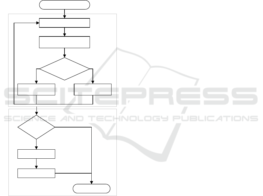
Figure 2: Flowchart of self-automated rule generation

mechanism implemented in SaFIN.

SaFIN also employs a self-automated rule

generation mechanism which formulates and updates

the rule base accordingly over time as depicted in

Figure 2. Upon achieving fuzzy partitioning of data

with CLIP, the rule base is ready to be formulated.

Rule generation runs in two stages, rule creation and

rule consistency check. For each incoming training

tuple, a novelty check is conducted between the new

data and its best matched fuzzy cluster, a new rule is

then added into the rule-base if determined to be

novel. Weights are also assigned to each rule as the

allocated weight is important in depicting each rules

significance while allowing the system to remove any

low impact or conflicting rules. Consistency checks

are performed upon rule-base formation for

inconsistent rule-base, which can be rules with

similar precedent conditions but with varying

outcomes. When inconsistency is found, the rule with

the lower weightage will be removed. This method

provides the rule pruning capability in SaFIN where

inconsistent and obsolete rules is removed over time.

3 METHODOLOGY

3.1 Study Site and Data Used

Dandenong catchment (Catchment 1) with an area of

about 272 km² is chosen as the study site which is

located in South East of Melbourne, Australia (See

Figure 3). The primary creek in this catchment is the

Dandenong creek which originates from the

Dandenong Ranges National Park and discharges into

Port Phillip Bay via both Mordialloc Creek and

Patterson River. Although farmlands as well as some

forest pockets remain in the catchment,

approximately 45% of the land has been overcome by

urbanization. Also, industrial activities are carried

extensively in large areas of the catchment. Eleven

years of daily rainfall and river discharge readings

from January 2005 to December 2015 from stations

Dandenong, Rowville, and Heathmont are used in this

study where Rowville and Heathmont are the two

upstream stations with Heathmont having the highest

elevation.

Sungai Kayu Ara river basin (Catchment 2) is

situated in a largely flattened urban landscape in

Selangor, Malaysia, and covers an area of 23.22 km²

(See Figure 4). The river basin is located within the

equatorial zone which is subjected to northeast and

southwest monsoon seasons. Annual mean rainfall

within the region is more than 2000mm while average

daily temperatures ranges from 25˚C to 33˚C. The

annual average evaporation rate for the basin is

estimated at 4 to 5mm per day, while mean monthly

relative humidity falls within 70% to 90%. The basin

consists 10 rainfall station and 1 river discharge

station. 40 rainfall-runoff events with 10-minutes

time series were extracted from the rainfall stations

spanning between March 1996 and July 2004.

Start

Incoming training tuple [x,d]

Find the best matched clusters

Is the newly created rule

novel?

Enhance weightage

Insert new rule;

Initialize weightage

Yes No

Is the created

rulebase consistent?

Delete inconsistent rules

Delete orphanedlabels

End

Yes

Rule Creation

Consistency Check

IJCCI 2018 - 10th International Joint Conference on Computational Intelligence

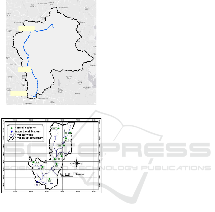
Figure 3: Schematic layout of Dandenong catchment.

Figure 4: Schematic layout of Sungai Kayu Ara river basin.

3.2 Physically-based Model Used

3.2.1 Storm Water Management System

(SWMM)

Storm Water Management System (SWMM) is a

dynamic rainfall-runoff simulation model developed

by the United States Environmental Protection

Agency (US EPA) used in conducting runoff quantity

and quality simulations. SWMM conceptualizes

physical elements of a watershed system into a

standard set of modelling objects where rain gauges

and sub-catchments are the principal objects used to

model the rainfall-runoff process. Each sub-

catchment is further subdivided into impervious and

pervious regions for simulating precipitation,

evaporation and infiltration losses. Using kinematic

wave equation, SWMM simulates the runoff based on

the physical routing of runoff through a system of

pipes and channels through a collective sub-

catchment area resulted by precipitation. The

kinematic equation is typically used in rainfall-runoff

modelling in which the model solves the continuity

equation along with a simplified form of the

momentum equation, allowing variations in spatial

and temporal flows within a conduit.

SWMM is one of the most widely used model in

a variety of hydrologic applications which includes

urban sewer planning, rainfall-runoff modelling, and

stormwater quality modelling. The model allows

flexibility of adjusting over 150 different constants

and coefficients which are physical dimensions,

impervious observations, soil properties and pipe

characteristics.

3.2.2 Hydrologic Engineering Center -

Hydrologic Modelling System

(HEC-HMS)

HEC-HMS is a lumped conceptual model in

hydrological applications. It attempts to simulate the

physical processes within the rainfall-runoff response

of a river basin system to a precipitation input through

conceptualizing the entire river basin as a system that

is interconnected by hydrologic and hydraulic

components like river basins, streams and reservoirs.

HEC-HMS is designed to be light in computational

complexity but flexible for a wide range of

geographic areas with different environment and

climates. The model includes many of the processes

involved in water circulation in the basin, such as,

precipitation, evaporation or infiltration. As such, the

model is widely used in many studies involving water

resources.

HEC-HMS requires pre-processing through HEC-

GeoHMS (Geospatial Hydrologic Modelling). HEC-

GeoHMS is an extension of ArcGIS which is

specifically designed for surface delineation and

producing the required geospatial data for HEC-HMS

hydrologic modelling. A surface Digital Elevation

Model (DEM) was used to extract drainage paths and

watershed boundaries to represent the hydrologic

structure used for simulating the watershed response

to precipitation. Results produced by HEC-GeoHMS

is then extracted and exported into HEC-HMS for

watershed hydrologic modelling.

3.3 Adaptive Network-based Fuzzy

Inference System (ANFIS)

ANFIS combines the reasoning capabilities of fuzzy

Rowville

Heathmont

Dandenong

Esri, HERE, DeLorme, MapmyIndia, © OpenStreetMap contributors, and the GIS user community

Rainfall-runoff Modelling in a Semi-urbanized Catchment using Self-adaptive Fuzzy Inference Network

systems with the learning mechanism of neural

networks. ANFIS was first developed by Jang (1993)

who implemented the Takagi-Sugeno fuzzy rules in a

five-layer neural network. Figure 5 shows the typical

structure of an ANFIS model for the case of 2 inputs.

Figure 5: Typical ANFIS structure for 2 inputs.

Further details about each layer and the

corresponding variables can be found in Talei et al.

(2010b). ANFIS has been successfully used in several

engineering applications including rainfall-runoff

modelling; therefore, it has been chosen as a

benchmark model in this study for comparison

purposes.

3.4 Input Data Selection and Model

Development

In Catchment 1, 11 years rainfall-runoff time series

were split into 2 datasets. The first 8 years was used

as training (calibration) dataset while the remaining 3

years of the data was used as validation dataset. The

input selection was conducted on training data set

where totally 6 rainfall antecedents of R

(t), R

(t-

1), R

(t), R

(t-1), R

(t), and R

(t-1) and 4 discharge

antecedents of Q

(t), Q

(t-1), Q

(t), Q

(t-1) were

considered as candidate inputs. It is worth mentioning

that R

, R

are rainfall at Dandenong, Rowville,

and Heathmont stations, respectively while Q

, Q

are upstream discharge at Rowville and Heathmont

stations, respectively; t is the present time and t-1 is

considered as a one-day lag. For Catchment 2, 40

event-based data were split into 12 training events

and 28 testing events. The rainfall-runoff dataset

consists of a total of 10 rainfall antecedents and 1

river discharge output, Q(t). The 10 rainfall

antecedents ranges from R1 to R10, where the

position of each respective rainfall station is shown in

Figure 4.

An input selection analysis was applied on both

catchments rainfall and discharge antecedents in

order to determine the choice of inputs for modelling.

As with most data driven models, the selection of

inputs is necessary to ascertain inputs that are better

associated with the discharge consequent to attain

greater efficacy during modelling. A hybridization of

both correlation analysis and mutual information

analysis proposed by Talei and Chua (2012) is

adopted in this study to select the inputs. This

approach prioritizes the inputs that have high

correlation with the output while possessing low

mutual information with other inputs. The Pearson

correlation coefficient is obtained by:

 

  

   















yyxx

yxC





(1)

in which



is the covariance between variables x

and y;



and



are the standard deviations of x and

y, respectively;

and

are the average values of x

and y, respectively, and n is the number of data points.

On the other hand, mutual information of two

variables x and y, MI(x,y) is calculated by:

 















yxMI





log

(2)

where



and



are the variance of the two variables

x and y, respectively and



is the covariance

between variables x and y.

3.5 Performance Criteria

In order to evaluate the models’ performance, four

different statistical measures are considered in this

study.

3.5.1 Nash-Sutcliffe Coefficient of Efficiency

(CE)

Coefficient of efficiency can be obtained by:

 

Obs i Sim i

Obs i Obs











(3)

where

iObs

and

iSim

are the observed and

simulated discharge values (in m

/s) for the ith data

point, respectively;

Obs

is the average value of the

observed discharge while n is the total number of data

points. It is worth mentioning that CE varies in the

IJCCI 2018 - 10th International Joint Conference on Computational Intelligence

domain of (-∞, 1] and is used to assess the goodness-

of-fitness between observed and simulated discharge

values of this study.

3.5.2 Coefficient of Determination (R

)

Coefficient of determination which measures the

degree of co-linearity between observed and

simulated values, varies in the range of [0, 1]. Value

of 1 indicates the perfect positive association while

the value of zero indicates no association. This

measure can be calculated by:

  

   



























SimiSim

ObsiObs

SimiSimObsiObs

QQQQ

(4)

where

iObs

and

iSim

are the observed and

simulated discharge values (in m

/s) for the ith data

point, respectively;

Obs

and

Sim

are the average

value of the observed and simulated discharge,

respectively, while n is the total number of data

points.

3.5.3 Root Mean Squared Error (RMSE)

RMSE accords extra importance on the outliers in

the data set and is therefore biased towards errors in

the simulation of high flow rates.

 

iObsiSim









RMSE

(5)

where

iObs

and

iSim

are the observed and

simulated discharge values (in m

/s) for the ith data

point, respectively; n is the total number of data

points.

3.5.4 Mean Absolute Error (MAE)

MAE is the average of all deviations from the original

data regardless of their sign. This parameter does not

allocate any weight to errors in extreme values. MAE

can be calculated by:

iObsiSim









MAE

(6)

where

iObs

and

iSim

are the observed and

simulated discharge values (in m

/s) for the ith data

point, respectively; n is the total number of data

points.

3.5.5 Relative Peak Error (RPE)

Peak estimation in rainfall-runoff modelling is a very

sensitive tasks since this measure is dealing with

extreme events. In this study, RPE is adopted to

evaluate the models’ capability in predicting peak

values. RPE is defined as:

   

Obsp

SimpObsp

RPE





(7)

where

Obsp

and

Simp

are the observed and

simulated peak discharge. Values closer to zero

indicate better estimation of peak flows.

4 RESULTS AND DISCUSSION

4.1 Dandenong Catchment (Catchment

Based on input selection analysis the best

combination of inputs was found to be of R

(t-1),

(t), Q

(t). Both SaFIN and ANFIS model was

calibrated using the same training data and input

combination. In addition, SWMM was also calibrated

using 1 arc-second resolution DEM data as well as

rainfall data from 9 different rainfall gauges. Further

comparisons were made through benchmarking

against results obtained from the autoregressive

model with exogenous inputs (ARX) model. ARX is

a linear regression model for input-output mapping.

In R-R modelling, ARX model output, Q(t) is

assumed to be related to rainfall antecedents, R(t-i)

and past outputs Q(t-i) by the following formula:

 







tejntRbitQatQ

)()1()(

(8)

where n

and n

are the number of past outputs and

inputs respectively, n

is the delay associated with

each input, e(t) is the true error term; and a

and b

are

model parameters to be optimized. To determine the

optimal model parameters, model fit is evaluated

using three residual statistics which are RMSE,

Akaike Information Criterion (AIC) (Akaike, 1974)

and Bayesian Information Criterion (BIC) (Rissanen,

1978). AIC and BIC are denoted by:

poi

2nRMSE)ln(nAIC 



(9)

Rainfall-runoff Modelling in a Semi-urbanized Catchment using Self-adaptive Fuzzy Inference Network

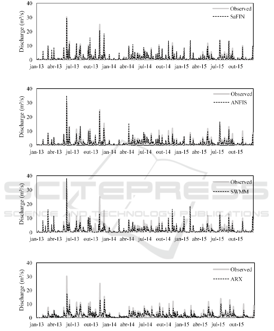
Figure 6: Observed versus simulated hydrograph in Catchment 1 by (a) SaFIN, (b) ANFIS, (c) SWMM and (d) ARX.

(a)

(b)

(c)

(d)

IJCCI 2018 - 10th International Joint Conference on Computational Intelligence

Figure 7: Scatterplots of observed versus simulated discharge in Catchment 1 by (a) SaFIN, (b) ANFIS, (c) SWMM and (d)

ARX.

)ln(nRMSE)ln(nBIC

poi oi



(10)

where 𝑛

𝑖−𝑜

is the number of input-output patterns and

𝑛

𝑝

is the number of model parameters. ARX was

employed with through varying range of values for

parameters n

, n

The model performance of all 4 models were then

compared using several performance metrics

including coefficient of efficiency (CE), R², RMSE,

and MAE as provided in Table 1.

Table 1: Performance of different models in Catchment 1.

Model

R²

RMSE

MAE

SaFIN

0.893

0.900

0.893

0.468

ANFIS

0.841

0.842

1.087

0.527

SWMM

0.686

0.696

1.532

0.671

ARX

0.417

0.421

1.174

0.550

As it can be seen, SaFIN was able to outperform

ANFIS, SWMM and ARX models for all

performance indices. Although SaFIN and ANFIS

models used data from 3 rainfall stations compared to

the 9 that was used to develop SWMM, both models

were able to outperform SWMM. However, it should

be noted that both SaFIN and ANFIS had the

advantage of having upstream discharge data as

inputs which contributes to performance

improvement. For further comparison, the observed

hydrograph is compared with the simulated ones by

SaFIN, ANFIS, SWMM and ARX as shown in Figure

6. As can be seen, all models were able to simulate

various ranges of flow in the testing dataset. To

evaluate the performance of the models in peak

estimation, the RPE metric was calculated for peak

discharge values greater than 10 m³/s (total 27 peaks).

(a)

(b)

(c)

(d)

Rainfall-runoff Modelling in a Semi-urbanized Catchment using Self-adaptive Fuzzy Inference Network

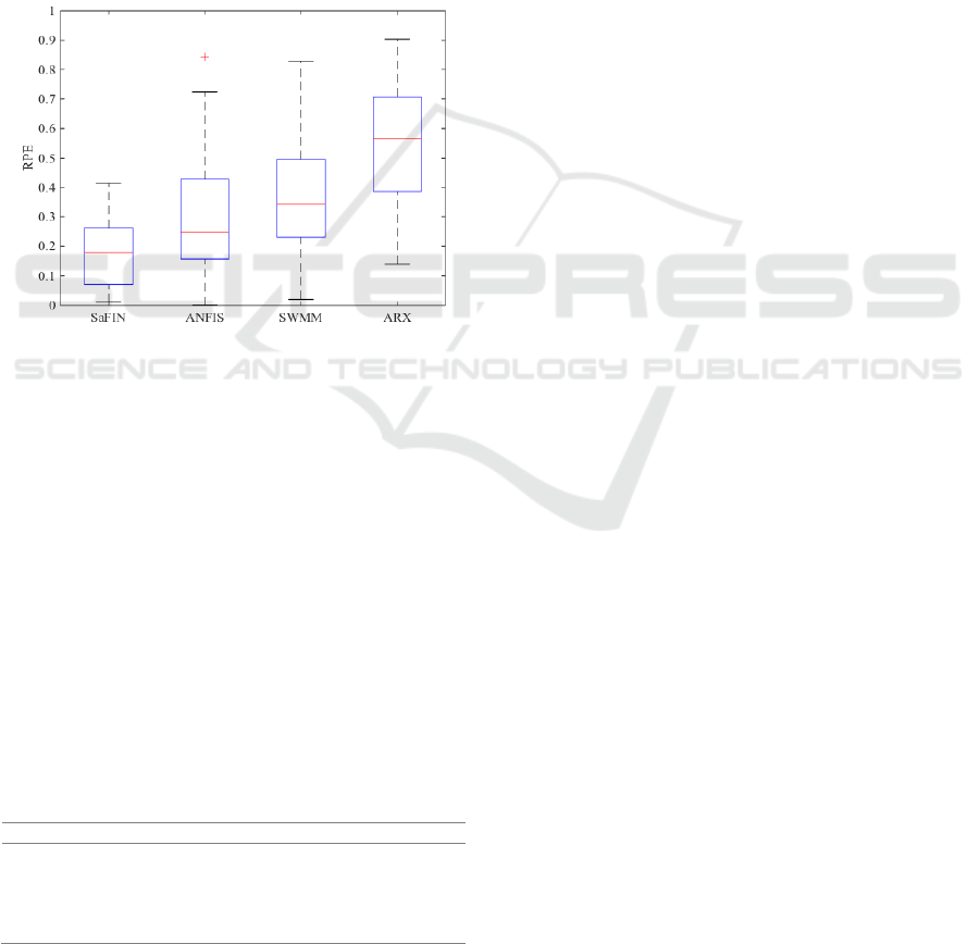
Figure 7 shows the scatterplots for each of the 4

model simulations. The scatterplots produced by

SaFIN and ANFIS appear to have an almost similar

spread in simulating low flows while ANFIS shows

more underestimations and overestimations for

higher flows values. Whereas the SWMM scatterplot

shows a wider spread when compared to SaFIN and

ANFIS.

Figure 8 shows the boxplots of the RPE values

obtained from SaFIN, ANFIS, SWMM and ARX. As

can be seen, SaFIN has the lowest median value and

the least range of errors when compared to the other

models followed by ANFIS and SWMM model. ARX

was the worst among these four models in the peak

estimation.

Figure 8: RPE boxplots for SaFIN, ANFIS, SWMM and

ARX in Catchment.

4.2 Sungai Kayu Ara River Basin

(Catchment 2)

SaFIN and ANFIS were both trained and tested using

inputs R1(t-7), R3(t-8), R5(t-7) and Q(t-1) that were

obtained from input selection analysis. It is worth

mentioning that R

refers to the ith rainfall station. The

results were compared against the ones obtained by

HEC-HMS from a study conducted by Alaghmand et

al. (2010). Additionally, ARX was used as an

additional benchmark to represent a linear regression

model. The averaged performance criteria across 28

testing datasets for all 4 models were compared and

shown in Table 2.

Table 2: Performance of different models in Catchment 2.

Model

R²

RMSE

MAE

SaFIN

0.851

0.868

3.201

3.021

ANFIS

0.824

0.829

3.425

3.275

HEC-HMS

0.743

0.862

3.813

3.261

ARX

0.423

0.501

8.552

8.794

From the averaged results, SaFIN outperformed

ANFIS, HEC-HMS and ARX in all performance

measures. ANFIS marginally underperformed as

compared to SaFIN, while the linear regression model

fails to model the highly non-linear nature of rainfall-

runoff modelling. Although both neuro-fuzzy models

were capable of performing better than the physical

model and linear regression models, it is worth noting

that SaFIN and ANFIS were trained and tested using

discharge antecedents with a lag of one timestep.

Figure 9 shows the boxplots of performance criteria

across 28 testing datasets simulated in catchment 2 by

the 4 models of this study. As it can be seen, SaFIN

boxplots show a consistently low spread across all

performance criteria. Additionally, SaFIN was able to

simulate peak discharge values more accurately and

consistently when compared to the other models.

Figure 10 shows the scatterplots of observed

versus simulated discharge for all 4 models. SaFIN

shows a relatively good performance in low and high

discharge values while having a larger spread in

simulating mid-peak discharges. Both ANFIS and

HEC-HMS show less consistency in simulating the

different categories of flow in this catchment when

compared to SaFIN. The simulated discharge

obtained from ARX model was consistently poor for

both low and high flows.

5 CONCLUSIONS

SaFIN R-R model with rule-pruning mechanism was

able to outperform an offline NFS model, ANFIS,

ARX model, and two physical models SWMM and

HEC-HMS in two different catchments in terms of

several goodness-of-fit indices. Moreover, it was

found that SaFIN significantly outperform ANFIS,

ARX, and the two physical models in peak

estimation. This study showed the great potential for

using SaFIN in Rainfall-Runoff modelling

application. SaFIN’s ability in updating its rule-base

was found as its major strength when compared to the

conventional NFS models with offline learning.

ACKNOWLEDGEMENTS

The authors would like to thank the Fundamental

Research Grant Scheme (FRGS) for providing

financial support for this research (grant number:

FRGS/1/2014/TK02/MUSM/03/1). This financial

support is provided by the Ministry of Higher

Education of Malaysia.

IJCCI 2018 - 10th International Joint Conference on Computational Intelligence

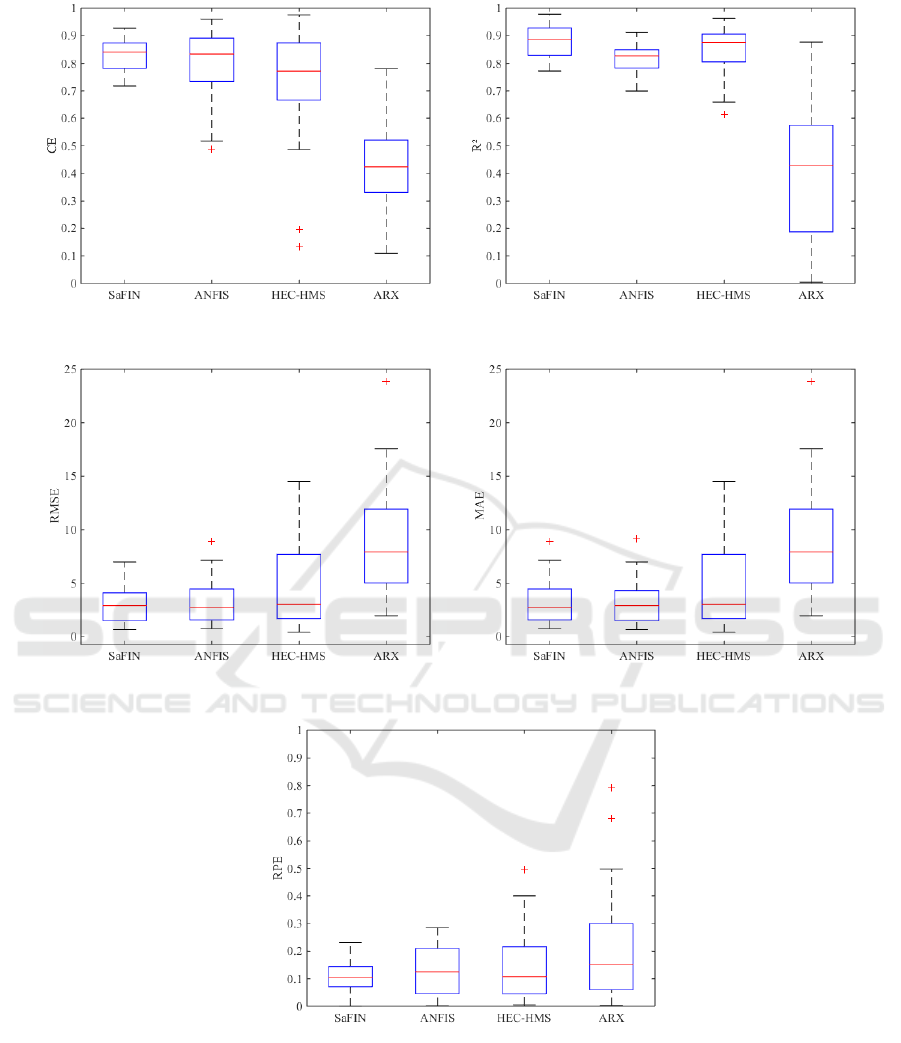
Figure 9: Boxplots of performance criteria: (a) CE, (b) R², (c) RMSE, (d) MAE and (e) RPE for SaFIN, ANFIS, HEC-HMS

and ARX models in Catchment 2.

(a)

(b)

(c)

(d)

(e)

Rainfall-runoff Modelling in a Semi-urbanized Catchment using Self-adaptive Fuzzy Inference Network

Figure 10: Scatterplots of observed versus simulated discharge in Catchment 2 by (a) SaFIN, (b) ANFIS, (c) HEC-HMS and

(d) ARX.

REFERENCES

Akaike, H. 1974. A new look at the statistical model

identification. Automatic Control, IEEE Transactions

on, 19, 716-723.

Alaghmand, S., Bin Abdullah, R., Abustan, I. & Vosoogh,

B. 2010. GIS-based river flood hazard mapping in

urban area (a case study in Kayu Ara River Basin,

Malaysia). Int. J. Eng. Technol, 2, 488-500.

Ashrafi, M., Chua, L. H. C., Quek, C. & Qin, X. 2017. A

fully-online Neuro-Fuzzy model for flow forecasting in

basins with limited data. Journal of Hydrology, 545,

424-435.

Bartoletti, N., Casagli, F., Marsili-Libelli, S., Nardi, A. &

Palandri, L. 2017. Data-driven rainfall/runoff

modelling based on a neuro-fuzzy inference system.

Environmental Modelling & Software.

Chang, T. K., Talei, A., Alaghmand, S. & Chua, L. H. 2016.

Rainfall-runoff modeling using dynamic evolving

neural fuzzy inference system with online learning.

Procedia Engineering, 154, 1103-1109.

Hong, Y.-S. T. 2012. Dynamic nonlinear state-space model

with a neural network via improved sequential learning

algorithm for an online real-time hydrological

modeling. Journal of hydrology, 468, 11-21.

Jang, J.-S. R. 1993. ANFIS: adaptive-network-based fuzzy

inference system. Systems, Man and Cybernetics, IEEE

Transactions on, 23, 665-685.

Luna, I., Soares, S. & Ballini, R. An adaptive hybrid model

for monthly streamflow forecasting. Fuzzy Systems

Conference, 2007. FUZZ-IEEE 2007. IEEE

International, 2007. IEEE, 1-6.

(a)

(b)

(c)

(d)

IJCCI 2018 - 10th International Joint Conference on Computational Intelligence

Minns, A. & Hall, M. 1996. Artificial neural networks as

rainfall-runoff models. Hydrological sciences journal,

41, 399-417.

Mukerji, A., Chatterjee, C. & Raghuwanshi, N. S. 2009.

Flood forecasting using ANN, neuro-fuzzy, and neuro-

GA models. Journal of Hydrologic Engineering, 14,

647-652.

Nayak, P., Sudheer, K., Rangan, D. & Ramasastri, K. 2005.

Short‐ term flood forecasting with a neurofuzzy model.

Water Resources Research, 41.

Nayak, P. C., Sudheer, K., Rangan, D. & Ramasastri, K.

2004. A neuro-fuzzy computing technique for modeling

hydrological time series. Journal of Hydrology, 291,

52-66.

Rajurkar, M., Kothyari, U. & Chaube, U. 2002. Artificial

neural networks for daily rainfall—runoff modelling.

Hydrological Sciences Journal, 47, 865-877.

Remesan, R., Shamim, M. A., Han, D. & Mathew, J. 2009.

Runoff prediction using an integrated hybrid modelling

scheme. Journal of hydrology, 372, 48-60.

Rissanen, J. 1978. Modeling by shortest data description.

Automatica, 14, 465-471.

Sajikumar, N. & Thandaveswara, B. 1999. A non-linear

rainfall–runoff model using an artificial neural network.

Journal of Hydrology, 216, 32-55.

Talei, A. & Chua, L. H. 2012. Influence of lag time on

event-based rainfall–runoff modeling using the data

driven approach. Journal of Hydrology, 438, 223-233.

Talei, A., Chua, L. H. C. & Quek, C. 2010a. A novel

application of a neuro-fuzzy computational technique

in event-based rainfall–runoff modeling. Expert

Systems with Applications, 37, 7456-7468.

Talei, A., Chua, L. H. C., Quek, C. & Jansson, P.-E. 2013.

Runoff forecasting using a Takagi–Sugeno neuro-fuzzy

model with online learning. Journal of Hydrology, 488,

17-32.

Talei, A., Chua, L. H. C. & Wong, T. S. 2010b. Evaluation

of rainfall and discharge inputs used by Adaptive

Network-based Fuzzy Inference Systems (ANFIS) in

rainfall–runoff modeling. Journal of Hydrology, 391,

248-262.

Tung, S. W., Quek, C. & Guan, C. 2011. SaFIN: A self-

adaptive fuzzy inference network. IEEE Transactions

on Neural Networks, 22, 1928-1940.

Xiong, L., Shamseldin, A. Y. & O'connor, K. M. 2001. A

non-linear combination of the forecasts of rainfall-

runoff models by the first-order Takagi–Sugeno fuzzy

system. Journal of Hydrology, 245, 196-217.

Zakhrouf, M., Bouchelkia, H. & Stamboul, M. 2015.

Neuro-Wavelet (WNN) and Neuro-Fuzzy (ANFIS)

systems for modeling hydrological time series in arid

areas. A case study: the catchment of Aïn Hadjadj

(Algeria). Desalination and Water Treatment, 1-13.

Rainfall-runoff Modelling in a Semi-urbanized Catchment using Self-adaptive Fuzzy Inference Network