
Effects of Longitudinal Shifts of Centre of Gravity on Ship Resistance: A
Case Study of a 31 M Hard-Chine Crew Boat
Ketut Suastika
1
∗
, Soegeng Riyadi
1
, I Ketut Aria Pria Utama
1
, and Xuefeng Zhang
2
1
Department of Naval Architecture, Institut Teknologi Sepuluh Nopember (ITS), Surabaya 60111, Indonesia
2
School of Marine Science and Technology, Tianjin University, Tianjin, China
Keywords:
CFD, Longitudinal Shift of Centre of Gravity, Hard-chine Crew Boat, Ship Resistance, Wave Pattern.
Abstract:
Computational fluid dynamics (CFD) simulations were performed to study effects of the longitudinal shifts
of centre of gravity (from the designed one) on ship resistance. Such a shift of centre of gravity has been
frequently observed in practice. This can occur, for example, due to inaccuracies in size and weight estimations
of ship components in the design stage and imperfections in bending, welding and assembly processes in the
production stage. For the reference case where there is no centre-of-gravity shift, the CFD results were verified
using data obtained from towing-tank experiments and using results from the Savitsky’s model. Results of
analysis show that for relatively low Froude numbers, a forward shift of centre of gravity results in a decrease
of ship resistance while a backward shift results in an increase of ship resistance. The opposite is true for
relatively high Froude numbers. Because the boat is designed to operate in relatively high Froude numbers
(Fr ¿ 0.7), a backward shift of centre of gravity is more favourable.
1 INTRODUCTION
In ship design, one of the owner requirements is the
ship speed. Based on the owner requirements, a ship
designer decides on the hull form and ship principal
particulars. So, ship speed enters the ship design pro-
cess in the first stage (EVANS, 1959). Estimations of
ship resistance and the required powering then follow.
In the first instance, the ship resistance is esti-
mated based on the full-load condition. However, a
ship is not always in full-load condition during its op-
erations. A shift of centre of gravity, particularly in
the longitudinal direction, may take place if the load-
ing condition changes. It has been observed that this
longitudinal shift of centre of gravity affects the ship
resistance (Kazemi and Salari, 2017).
A shift of centre of gravity, relative to the designed
one, can also take place during the production pro-
cess of the ship. This can happen due to, for example,
oversize of main engine, inaccuracy in weight estima-
tions of generator, structural components etc. In addi-
tion, a shift of centre of gravity can also occur due to
imperfections in bending, welding and assembly pro-
cesses (Takechi et al., 1998).
Figure 1 illustrates the production process of a
hard-chine crew boat in PT. Orela Shipyard, Ujung
Pangkah, Gresik, Indonesia and Figure 2 shows the
construction part near the bow. The boat in produc-
tion as shown in Figure 1 and 2 was made of alu-
minium. In such a production process, imperfections
as described above can occur, which result in a (lon-
gitudinal) shift of centre of gravity relative to the de-
signed one. Although longitudinal shifts of centre of
gravity have frequently been observed in practice, its
effects on ship resistance have insufficiently been ex-
plored.
The purpose of the present study is to investigate
effects of the longitudinal shifts of centre of gravity
on ship resistance. For that purpose, a hard-chine
crew boat, designed and built by PT. Orela Shipyard,
as shown in Figure 1 and 2, is considered as a case
study. The ship principal-particulars are summarized
in Table 1.
Computational fluid dynamics (CFD) simulations
were performed and the results for the reference case
without shift of centre of gravity were verified us-
ing data obtained from towing-tank experiments and
using results from the Savitsky’s model (Savitsky,
1964).
The research method is further elaborated in Sec-
tion. 2. The results and discussion are presented
in Section 3. The paper ends with conclusions, pre-
sented in Section 4.
Suastika, K., Riyadi, S., Utama, I. and Zhang, X.
Effects of Longitudinal Shifts of Centre of Gravity on Ship Resistance: A Case Study of a 31 m Hard-chine Crew Boat.
DOI: 10.5220/0008550801450152
In Proceedings of the 3rd International Conference on Marine Technology (SENTA 2018), pages 145-152
ISBN: 978-989-758-436-7
Copyright
c
2020 by SCITEPRESS – Science and Technology Publications, Lda. All rights reserved
145
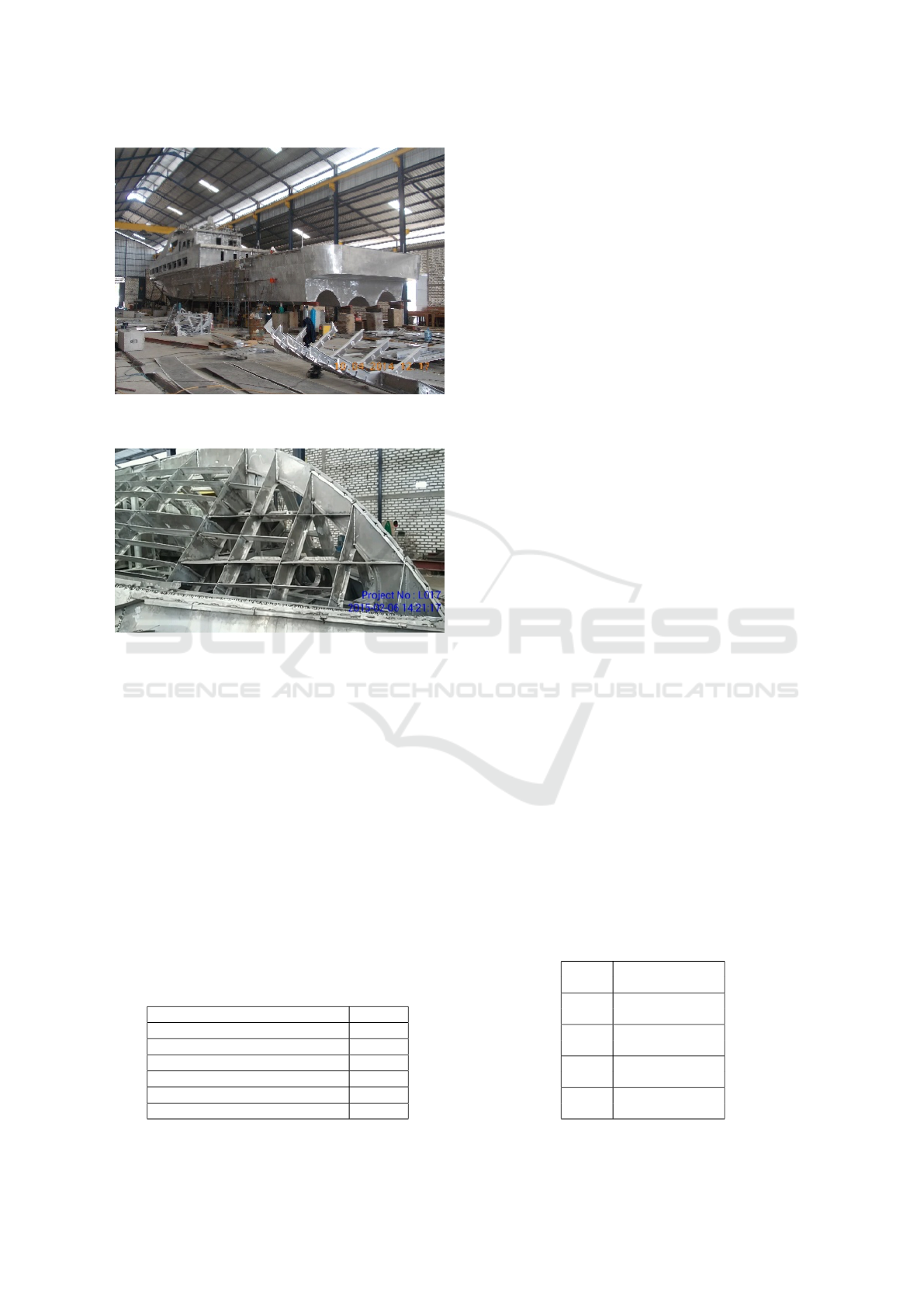
Figure 1: A Hard-chine Crew Boat during The Production
Process (courtesy of PT. Orela Shipyard).
Figure 2: Construction Part of The Hard-chine Orela Crew
Boat Near The bow (courtesy of PT. Orela Shipyard).
2 METHOD
Computational fluid dynamics (CFD) (Anderson,
1994; Versteeg et al., 1995; Moukalled et al., 2016)
are utilized to simulate effects of the longitudinal shift
of centre of gravity (relative to the designed one) on
ship resistance. Table 2 summarizes variations of po-
sition of the centre of gravity in the longitudinal di-
rection considered in the present study. As mentioned
above, for the reference case where there is no shift
of centre of gravity (Case 0), the CFD results are
verified using data obtained from towing-tank exper-
iments and using results from the Savitsky’s model
(Savitsky, 1964).
Table 1: Ship Principal-particulars of The Crew Boat.
Length Overall (LOA) 31.20 m
Length Between Perpendicular (L
PP
) 28.80 m
Breadth (B) 6.80 m
Depth (H) 2.75 m
Draft (T) 1.40 m
Maximum Speed (V
max
) 26 kn
Displacement (∆) 104.68 t
2.1 Towing-tank Experiments
Towing-tank experiments were performed at the Hy-
drodynamics Laboratory, Faculty of Marine Tech-
nology, Institut Teknologi Sepuluh Nopember (ITS),
Surabaya, Indonesia. The dimension of the tank is as
follows: length = 50.0 m, width = 3.0 m, maximum
water depth = 2.0 m and maximum towing speed =
4.0 m/s.
A model of the ship was built from fibreglass re-
inforced plastic (FRP) coated with paint and resin.
The geometrical scale between model and prototype
is 1:40. The Froude scaling was applied between the
full scale and model ship in the experiments. The ship
resistance was measured using a load cell. Before per-
forming a test, the load cell was calibrated by using a
mass of 0.5 kg.
The ship speeds tested were 11, 14, 17, 20, 23
and 26 knots (full-scale speed). These correspond to
model speeds of 0.894, 1.14, 1.38, 1.63, 1.87 and 2.11
m/s, respectively. The Froude-number range is ap-
proximately between 0.4 to 0.8. At Fr ¡ 0.5 the ship is
expected to reveal displacement characteristics while
at Fr ¿ 0.7 it is expected to reveal semi-displacement
characteristics. Figure 3 shows the ship model towed
at 20 kn (Fr = 0.62).
2.2 CFD Simulations
CFD simulations were performed to calculate the ship
resistance for varying ship speed and varying position
of centre of gravity. The speed variations are in ac-
cordance to the speeds measured in the towing-tank
experiments. The variations of centre-of-gravity po-
sition are as summarized in Table 2.
The CFD simulations utilized the software pack-
age Numeca Fine/Marine®(Marine Fine, 2013),
which is based on a finite volume method (FVM).
The ISIS-CFD code of the package solves the incom-
pressible unsteady Reynolds-averaged Navier-Stokes
(RANS) equations for modelling turbulent multi-
Table 2: Variations of Longitudinal Position of Centre of
Gravity Considered in The Study (measured from the aft
perpendicular).
Case 0
1.00 LCG (design)
12.45 m (+0.0m)
Case 1
1.03 LCG
12.85 m (+0.4m)
Case 2
1.02 LCG
12.65 m (+0.4m)
Case 3
0.98 LCG
12.25 m (-0.2m)
Case 4
0.97 LCG
12.05 m (-0.4m)
SENTA 2018 - The 3rd International Conference on Marine Technology
146

Figure 3: Ship Model of The 31 m Hard-chine Crew Boat
Towed at 20 knots (Fr =0.62).
phase flows with appropriate boundary conditions. It
utilizes the volume of fluid (VOF) method to resolve
the free surface boundary (Hirt and Nichols, 1981),
that is, modelling of the generation of waves. The
mass, momentum and volume-fraction conservation
equations are represented, respectively, as follows:
∂
∂t
Z
v
ρdV +
Z
S
ρ(U − U
d
) · ndS = 0 (1)
∂
∂t
Z
v
ρU
i
dV +
Z
S
ρU
i
(U − U
d
) · ndS
=
Z
s
(τ
i j
I
j
− pI
i
) · ndS +
Z
V
ρg
i
dV
(2)
∂
∂t
Z
v
c
i
dV +
Z
S
c
i
(U − U
d
) · ndS (3)
In Equation (1), (2) and (3), V is the control vol-
ume, bounded by the closed surface S with a normal
vector n directed outward moving at the velocity U
d
,
U is the velocity field and p is the pressure field. Fur-
thermore, τ
i j
is the turbulent (Reynolds) stress tensor,
g
i
is the component of the gravity vector, I
j
is a vec-
tor whose components are zero except for j=1 and c
i
is the volume fraction of fluid i and is used to distin-
guish the presence (c
i
= 1) and the absence (c
i
= 0) of
fluid i.
The turbulence model used is the SST k-ω model
(SST for shear-stress transport), where k is the turbu-
lent kinetic energy and ω is the specific dissipation
rate (Menter, 1994)(ISIS-CFD, 2013). The main fea-
ture of the model is zonal blending of modelling, us-
ing the Wilcox’s k-ω model for the flow near solid
walls and using the standard k-εmodel (transformed
into k-ω formulation) for the flow near boundary layer
edges and in free-shear layers. The transport equa-
tions for k and ω are represented as follows, where
the blending coefficient F
1
models the coefficients of
the original ω and eε.
Figure 4: A Sketch of The Computational Domain
∂
ρ
k
∂t
+
∂
∂x
j
ρU
j
k − (µ + σ
ω
µ
t
)
∂k
∂x
j
= τ
t
i j
S
i j
− βρωk
(4)
∂
ρ
ω
∂t
+
∂
∂x
j
ρU
j
ω − (µ + σ
ω
µ
t
)
∂ω
∂x
j
= P
ω
− βρω
2
+ 2(1 − F
1
)
ρσ
ω
2
ω
∂k
∂x
j
∂ω
∂x
j
(5)
Details of the model are described in (11). The
cell size near the wall, y
wall
, is calculated based on
the wall variable y
+
, which is given as follows:
y
+
=
ρu
t
y
wall
µ
(6)
where u
τ
=
q
τ
wall
ρ
=
q
1
2
ρ(V
2
re f f
)C
f
is the friction ve-
locity. The value of y
wall
is calculated as
y
wall
= 6
v
re f
ν
7/8
L
re f
2
1/8
y
+
(7)
In the simulations, the value for y
+
is set equal to
10 and the length between the perpendiculars (L
PP
) is
used as the reference length L
re f
.
The computational domain is sketched in Fig 4.
Due to symmetry, only a half of the ship is modelled.
The inlet is located at 1.0L upstream from the vessel,
while the outlet is located at 3.0L downstream from
the vessel. The side wall is 1.50L aside the vessel.
The bottom wall is located at 1.50L below the vessel
and the top wall is located at 0.50L above the ves-
sel (L is the length between the perpendiculars L
PP
).
The boundary conditions (according to the definitions
used in Numeca Fine/Marine®) are summarized in
Table 3.
It is well-known that, in the application of a nu-
merical method, there is a trade-off between accu-
Effects of Longitudinal Shifts of Centre of Gravity on Ship Resistance: A Case Study of a 31 m Hard-chine Crew Boat
147
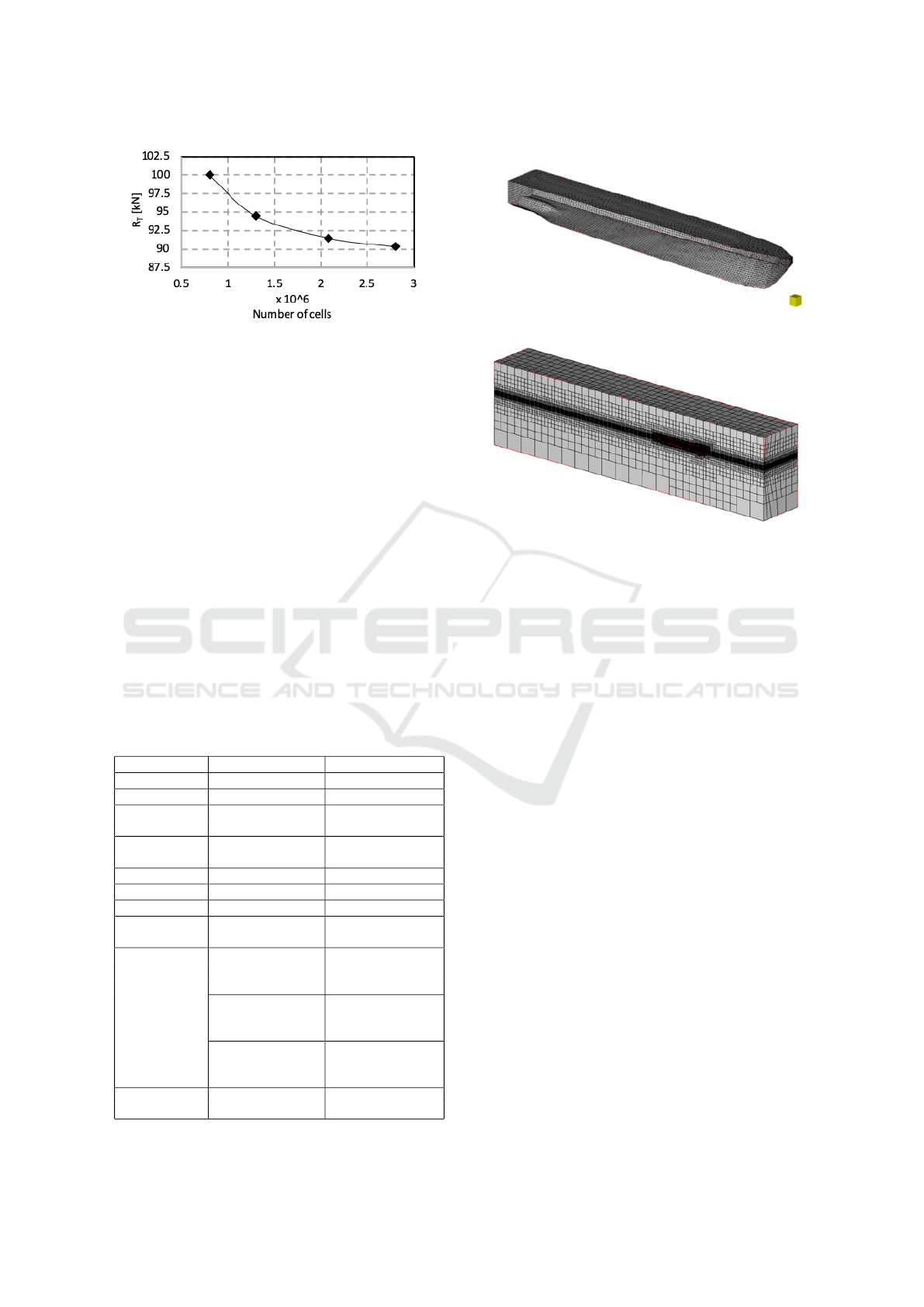
Figure 5: Total Ship Resistance as Function of Number of
Cells for Ship Speed of 20 knots (Fr = 0.62).
racy (which depends on the number of computa-
tional cells) and computational cost. To find an op-
timum number of cells used in the simulations, grid-
independence tests were performed as illustrated in
Figure 5. As shown in Figure. 5, the total ship resis-
tance decreases monotonically with increasing num-
ber of cells (elements). The total resistance is ex-
pected to reach an asymptotic value for very large
number of cells (theoretically, if the number of cells
tends to infinity). Due to the limited capacity of avail-
able hardware, the number of cells of 2.8 x 10⁶ was
considered as the most optimum number of cells in
the present study.
Results of the meshing are shown in Figure. 6 and
7, respectively, for (a half of) the ship hull and the
computational domain with the ship model therein.
The total number of cells in the latter case is 2.8 x
106. This number of cells has also been utilized in
Table 3: Boundary Conditions
Description Type Condition
Inlet (Xmin) EXT Far field, Vx = 0
Outlet (Xmax) EXT Far field, Vx = 0
Bottom (Zmin) EXT Update hydrostatic
pressure
Top (Zmax) EXT Update hydrostatic
pressure
Side (Ymin) MIR Mirror
Side (Ymax) EXT Far field, Vx = 0
Ship hull SOL Wall function
Ship deck SOL Free slip (zero
shear stress)
Motion
Translation in Speed = Ship speed,
X direction with using one half
a given speed sinusoidal ramp
Translation in Linear law
Z direction with
solved motion type
Rotation in Ry Linear law
(pitch) with
solved motion type
Convergence Order of magnitude Second order
criteria of residual decrease
Figure 6: Mesh of A Half of The Ship Hull.
Figure 7: Computational Domain with The Ship Model
Therein. The total number of cells is 2.8 x 10
6
.
a previous study utilizing the same crew boat where
effects of the application of a Hull Vane®on ship re-
sistance was studied (Riyadi and Suastika, 2018).
3 RESULTS AND DISCUSSIONS
To verify the CFD results, these are compared with
those obtained from Savitsky’s model and experimen-
tal data (towing-tank experiments). Figure 8 shows
a comparison of total ship resistance as function of
Froude number obtained from CFD, Savitsky’s model
(Savitsky, 1964) and towing-tank experiments for the
reference case (Case 0; see Table 2). For relatively
low Froude numbers (Fr ¡ 0.45) and for relatively
high Froude numbers (Fr ¿ 0.7), the CFD and Sav-
itsky’s results underestimate the experimental data.
The average relative error between the results of CFD
and Savitsky’s model (Savitsky, 1964) is 2.5% and
that between CFD results and towing-tank data is
2.9%, which are relatively small.
A hump region is observed in the Froude num-
ber range between approximately 0.45 and 0.70. In
this hump region the results from CFD and Savit-
sky’s model (Savitsky, 1964) overestimate the exper-
imental data. Furthermore, the CFD and Savitsky’s
results show the hump region more clearly than the
towing-tank results. However, generally, the three
curves show a similar trend. Such a hump region
SENTA 2018 - The 3rd International Conference on Marine Technology
148

Figure 8: Total Ship Resistance as Function of Froude
Number, obtained from CFD, Savitsky (Savitsky, 1964) and
Towing-tank Experiments.
Figure 9: Total Ship Resistance as Function of Froude
Number for the Five Cases as summarized in Table 2.
has been observed in earlier studies (Yousefi et al.,
2013)(Suastika et al., 2017) For Fr ¡ 0.45, the hydro-
static forces (weight and buoyancy) are dominant. On
the other hand, for Fr ¿ 0.7 the hydrodynamic force
becomes more dominant than the hydrostatic forces.
Effects of the longitudinal shifts of centre of grav-
ity on ship resistance are investigated using CFD sim-
ulations. In the simulations, the ship displacement is
kept constant.
Figure 9 shows the total ship resistance as function
of Froude number for the five cases as summarized in
Table 2. The difference in ship resistance from the
five curves as shown in Figure 9 is rather small and
difficult to be distinguished. To make the difference
clearer, Figure 10 shows the percentage of relative dif-
ference compared to the reference case (Case 0). As
shown in Figure 10, for relatively low Froude num-
bers (say Fr ¡ 4.5), a forward shift of centre of gravity
results in a decrease of ship resistance but a backward
shift results in an increase of ship resistance. On the
contrary, for relatively high Froude numbers (say Fr
¿ 0.6), a forward shift of centre of gravity results in an
increase of ship resistance but a backward shift results
in a decrease of ship resistance.
Figure 10: Relative Difference in Ship Resistance Com-
pared to The Reference Case (Case 0; LCG design).
Due to the shift of centre of gravity, the ship re-
sistance can increase approximately 6% in the lowest
Froude number (Case 3; LCG - 0.2 m) and approx-
imately 3% in the highest Froude number (Case 1;
LCG + 0.4 m). Furthermore, the decrease can reach
approximately 4% in the lowest Froude number (Case
2; LCG + 0.2 m) and approximately 2% in the high-
est Froude number (Case 3; LCG - 0.2 m and Case
4; LCG - 0.4 m). Which shift is more favourable, it
depends on the operational scheme of the boat. If,
in most of the time, it is operated at relatively large
speed (say Fr ¿ 0.6) then the backward shift of centre
of gravity is more favourable.
Figure 11 shows wave patterns for the different
cases as summarized in Table 2 with Fr = 0.34. Fig-
ure 12 shows locations of measurement points of free-
surface elevation (water level) near the ship hull. In
addition, Figure 13 shows wave patterns for the dif-
ferent cases with Fr = 0.80. The wave pattern for Fr =
0.34 is very different from that for Fr = 0.80 (compare
for example Figure 11a with Figure 13a), as may be
expected, because of the very different Froude num-
bers. For Fr = 0.34, two wave crests and two wave
troughs are observed along the ship while for Fr =
0.80 only one wave crest and one wave trough are ob-
served.
For Fr = 0.34, a forward shift of centre of gravity
(Case 1 and 2) results in a deeper wave trough in front
of the midship (points 3 and 4 in Figure 12) while
a backward shift results in a higher wave through in
front of the midship, compared to the reference case
(see also Table 4). Near the bow (points 1 and 2), a
forward shift results in an increase of water level but a
backward shift results in a decrease of the water level.
Furthermore, near the stern (points 9, 10 and 11), a
forward shift results also in an increase of water level
but a backward shift results in a decrease of the water
level.
For Fr = 0.80, a forward shift of centre of gravity
results in a higher wave trough in front of the mid-
Effects of Longitudinal Shifts of Centre of Gravity on Ship Resistance: A Case Study of a 31 m Hard-chine Crew Boat
149

(a) Case 0; Fr = 0.34
(b) Case 0(+0.4m); Fr = 0.34
(c) Case 0(+0.2m); Fr = 0.34
(d) Case 0(-0.2m); Fr = 0.34
(e) Case 0(-0.4m); Fr = 0.34
Figure 11: Contour of Water Surface Elevation (water level
η) for Different Cases as summarized in Table 2 with Fr =
0.34. The reference plane is at the base line (keel), which is
1.40 m below the mean water surface.
Figure 12: Locations of Measurement Points of Free Sur-
face Elevation (water level) near the Ship Hull.
Table 4: Water Level η at The Measurement Points as
shown in Figure 12, Relative to The Water Level for The
Reference Case (Case 0) η
0
The Reference Horizontal
Plane is at The Base Line, which is 1.40 m below The Mean
Water Surface. The Froude Number Fr = 0.34.
Point Case 0
η
0
[m]
Case 1
η − η
0
[m]
Case 2
η − η
0
[m]
Case 3
η − η
0
[m]
Case 4
η − η
0
[m]
1 1.52 0.00 0.00 0.00 -0.01
2 1.45 +0.01 +0.01 0.00 0.00
3 1.09 -0.01 -0.01 +0.01 +0.03
4 1.16 -0.02 -0.02 0.00 +0.01
5 1.25 0.00 +0.01 -0.01 0.00
6 1.40 0.00 0.00 0.00 0.00
7 1.35 0.00 +0.01 -0.01 0.00
8 1.26 0.00 0.00 +0.01 +0.01
9 1.21 +0.05 +0.03 -0.01 -0.03
10 1.39 +0.03 +0.02 -0.01 -0.02
11 1.45 +0.02 +0.01 -0.02 -0.02
ship (points 3 and 4 in Figure 12) while a backward
shift results in a lower wave through compared to the
reference case (see Table 5). This is also the case for
the region near the bow (points 1 and 2), that is, an
increase of water level due to a forward shift but a de-
crease of water level due to a backward shift. Behind
the midship (points 5, 6 and 7), a forward shift results
in a decrease of water level while a backward shift
Table 5: Water Level η at The Measurement Points as
shown in Figure 12, Relative to The Water Level for The
Reference Case (Case 0) η
0
The Reference Horizontal
Plane is at The Base Line, which is 1.40 m below The Mean
Water Surface. The Froude Number Fr = 0.34.
Point Case 0
η
0
[m]
Case 1
η − η
0
[m]
Case 2
η − η
0
[m]
Case 3
η − η
0
[m]
Case 4
η − η
0
[m]
1 1.45 +0.01 0.00 0.00 -0.01
2 1.43 0.00 0.00 0.00 -0.01
3 1.78 +0.03 +0.01 -0.01 -0.03
4 1.59 +0.03 +0.02 -0.01 -0.01
5 1.52 -0.01 -0.01 +0.01 0.00
6 1.37 -0.05 -0.03 +0.03 +0.05
7 1.42 -0.03 -0.02 +0.02 +0.06
8 1.56 0.00 0.00 -0.01 0.00
9 0.76 +0.03 +0.01 -0.01 -0.02
10 0.86 0.00 -0.01 +0.01 +0.03
11 0.79 0.00 0.00 0.00 +0.01
SENTA 2018 - The 3rd International Conference on Marine Technology
150

(a) Case 0; Fr = 0.8
(b) Case 0(+0.4m); Fr = 0.8
(c) Case 0(+0.2m); Fr = 0.8
(d) Case 0(-0.2m); Fr = 0.8
(e) Case 0(-0.4m); Fr = 0.8
Figure 13: Contour of Water Surface Elevation (water level
η) for Different Cases as summarized in Table 2 with Fr =
0.8. The reference plane is at the base line (keel), which is
1.40 m below the mean water surface.
results in an increase of water level.
A forward shift of centre of gravity results in a
different wave pattern compared to a backward shift.
This difference of wave pattern results in different
wave resistance, which ultimately affects the total re-
sistance as discussed above. The above observations
characterize the hull form of the hard-chine crew boat.
4 CONCLUSIONS
CFD simulations were performed to study effects of
the longitudinal shifts of centre of gravity on ship re-
sistance. For the reference case where there is no
centre-of-gravity shift, the CFD results are verified
using data from towing-tank experiments and results
from the Savitsky’s model (Savitsky, 1964). Centre-
of-gravity shifts can occur in practice due to, for ex-
ample, oversize of main engine, inaccuracy in weight
estimations of generator, structural components etc. It
can also occur due to imperfections in bending, weld-
ing and assembly processes.
For relatively low Froude numbers (say Fr ¡ 4.5),
where the hydrostatic forces are dominant, a forward
shift of centre of gravity results in a decrease of ship
resistance but a backward shift results in an increase
of ship resistance. On the contrary, for relatively high
Froude numbers (say Fr ¿ 0.6), where the hydrody-
namic forces are dominant, a forward shift of centre
of gravity results in an increase of ship resistance but a
backward shift results in a decrease of ship resistance.
It depends on the operational scheme of the ship
which longitudinal shift of centre of gravity is more
favourable. In the present case, where the boat is de-
signed to operate in a semi-planing mode (Fr ¿ 0.7), a
backward shift of centre of gravity is more favourable.
The wave pattern for relatively low Froude num-
bers (Fr ¡ 0.45) is very different from that for rela-
tively high Froude numbers (Fr ¿ 0.7). For relatively
low Froude numbers, two wave crests and two wave
troughs were observed along the ship while for rela-
tively high Froude numbers only one wave crest and
one wave trough were observed.
A forward shift of centre of gravity results in a
different wave p]attern compared to a backward shift.
This difference of wave pattern results in different
wave resistance, which ultimately affects the total
ship resistance. The resulting wave pattern is char-
acteristic for the hull form being investigated.
Effects of Longitudinal Shifts of Centre of Gravity on Ship Resistance: A Case Study of a 31 m Hard-chine Crew Boat
151

ACKNOWLEDGEMENTS
Ketut Suastika was a visiting researcher at the School
of Marine Science and Technology, Tianjin Univer-
sity, China, in the period from October 10th, 2018 to
January 9th, 2019 where parts of the present study
were carried out. He thanks the School of Marine Sci-
ence and Technology, Tianjin University, China, for
the opportunity having been provided. This research
project was supported by the Ministry of Research,
Technology and Higher Education (Ristekdikti) of the
Republic of Indonesia, under the grant Penelitian Ter-
apan Unggulan Perguruan Tinggi (PTUPT) with con-
tract no. 1031/PKS/ITS/2018.
REFERENCES
Anderson, J. D. (1994). Computational fluid dynamics : the
basics with applications. McGraw-Hill, New York.
EVANS, J. H. (1959). BASIC DESIGN CONCEPTS. Jour-
nal of the American Society for Naval Engineers,
71(4):671–678.
Hirt, C. W. and Nichols, B. D. (1981). Volume of fluid
(VOF) method for the dynamics of free boundaries.
Journal of Computational Physics Journal of Compu-
tational Physics, 39(1):201–225.
ISIS-CFD (2013). Theoretical Manual. EMN, Ecole Cen-
trale de Nantes.
Kazemi, H. and Salari, M. (2017). Effects of Loading Con-
ditions on Hydrodynamics of a Hard-Chine Planing
Vessel Using CFD and a Dynamic Model. Interna-
tional Journal of Maritime Technology, 7(0):11–18.
Marine Fine (2013). User Manual Flow Integrated Envi-
ronment for Marine Hydrodynamic. Numeca Interna-
tional, Belgium.
Menter, F. R. (1994). Two-Equation Eddy-Viscosity Tur-
bulence Models for Engineering Applications. AIAA
journal., 32(8):1598.
Moukalled, F., Mangani, L., and Darwish, M. (2016). The
Finite Volume Method in Computational Fluid Dy-
namics : an Advanced Introduction with OpenFOAM
and Matlab. Springer.
Riyadi, S. and Suastika, K. (2018). Experimental and nu-
merical study of high Froude-number resistance of
ship utilizing a Hull Vane®: A case study of a hard-
chine crew boat. In Proc.11th International confer-
ence on marine technology. MARTEC.
Savitsky, D. (1964). Hydrodynamic Design of Plan-
ing Hulls. Marine Technology and SNAME News,
1(04):71–95.
Suastika, K., Hidayat, A., and Riyadi, S. (2017). Effects
of the application of a stern foil on ship resistance: A
case study of an orela crew boat. International Journal
of Technology, 8:1266.
Takechi, S., Aoyama, K., and Nomoto, T. (1998). Basic
studies on accuracy management system based on es-
timating of weld deformations. Journal of the Society
of Naval Architects of Japan, 3:194–200.
Versteeg, H., Malalasekera, W., Orsi, G., Ferziger, J. H.,
Date, A. W., and Anderson, J. D. (1995). An Intro-
duction to Computational Fluid Dynamics - The Finite
Volume Method.
Yousefi, R., Shafaghat, R., and Shakeri, M. (2013). Hydro-
dynamic analysis techniques for high-speed planing
hulls. Applied Ocean Research, 42:105–113.
SENTA 2018 - The 3rd International Conference on Marine Technology
152
