The Finite Volume Method Applied to The Patlak-Keller-Segel

Chemotaxis Model in a General Mesh

Ouafa Soualhi

and Mohamed Rhoudaf

Department of Mathematics, Moulay Ismail University, Meknes, Morocco

Keywords:

chemotaxis; ﬁnite volume; numerical simulation.

Abstract:

In this paper, we present the discrete duality ﬁnite volume method (DDFV) applied to a model of (Patlak)

Keller-Segel modeling chemosensitive movements, this model consists of a coupled system of elliptic and

parabolic equations. Firstly, we prove the existence and uniqueness of the numerical solution to the proposed

scheme. Next, numerical simulations are performed to verify accuracy.

1 INTRODUCTION

Chemotaxis is the characteristic movement or orienta-

tion of cells, organisms or bacteria along chemical con-

centration gradient towards chemoattractant or away from

chemorepellant, it is very essential for organisms to search

food around them. Well-known examples, the ﬁrst is the

bacteria Escherichia Coli such that there cells are known to

swim towards the amino acids serine and aspartic acid and

towards sugars such as maltose, ribose, galactose and glu-

cose, the second is the amoeba Dycliostelium discoideum

,where it has been used as a model organism in molecu-

lar biology and genetics, and is studied as an example of

cell communication, differentiation, and programmed cell

death.

There are two types of chemotaxis:

1) Positive chemotaxis: the movement of organisms to-

wards a chemical.

2) Negative chemotaxis: the movement of organisms away

from a chemical.

Patlak in 1953 (Patlak, 2953) and Keller and Segel in

1970 (Keller and Segel, 1970), were created as a classical

model to describe the evolution over time of the cell den-

sity n(x,t) and the chemical signal concentration variable

S(x,t) assuming that the cells emit directly the chemoat-

tractant which is directly diffused. A lot of theoretical and

mathematical model chemotaxis phenomena but the most

famous model is the following the classical Paltak-Keller-

Segel(PKS) system:

(

∂n

∂t

− div(∇n − χn∇S) = 0, on Ω × [0,T ],

−div(∇S) − µn + S = 0, on Ω × [0,T ],

(1)

where

χ : The chemotactic sensitivity function.

µ : The secretion rate at which the chemical substance is

emitted by the cells, let µ > 0.

Ω is a Convex, bounded and open set of R

and T > 0.

The initial conditions on Ω are given by

n(x,0) = n

(x), in Ω. (2)

Therefore, the system (1) is supplemented by the following

boundary conditions on ∂Ω × [0,T ].

∇n.ν = 0, in ∂Ω × [0, T ], (3)

∇S.ν = 0, in ∂Ω × [0, T ], (4)

with ν is the unite vector.

This model is very successful for describing the aggre-

gation of the population in a ﬁnite time point-wise blowup

(in a single point).

In the literature, there exist several works present

some numerical method to solve the classical Keller-Segel

system, let us set: F. Filbet prove the existence and

uniqueness of a numerical solution to the scheme ﬁnite

volume schemes in (G.Chamoun and R.TalhoukF.Filbet,

2006) and the authors present the ﬁnite volume scheme

for a Keller-Segel model with additional cross-diffusion in

(Bessemoulin-Chatard and Jungel, 2014). In (A.J.Carrillo,

2012) the authors present the cross diffusion and nonlinear

diffusion preventing blow up in the Keller-Segel model.

A second-order positivity preserving central-upwind

scheme is presented by A. Chertock and A. Kurganov in

(A.Chertock and A.Kurganov, 2008) for chemotaxis and

haptotaxis models. Noted that, the fully discrete analysis

of a discontinuous ﬁnite element method in (Ref, a) and

the new interior penalty discontinuous Galerkin methods

in (Ref, b). Moreover, (Ha

skovec and Schmeiser, 2009;

skovec and Schmeiser, 2011) propose the numerical

and theoretical study of the stochastic particle approxi-

mation and the paper (A.Marrocco, 2003) concerned the

numerical simulation of chemotactic using the mixed ﬁnite

elements method. Finite-element method for a simpliﬁed

Keller-Segel system in (N.Saito, 2007; N.Saito, 2012) and

ﬁnite difference schemes to a parabolic-elliptic system

modelling chemotaxis in (N.Saito and T.Suzuki, 2005). An

Soualhi, O. and Rhoudaf, M.

The Finite Volume Method Applied to The Patlak-Keller-Segel Chemotaxis Model in a General Mesh.

DOI: 10.5220/0009775800420049

In Proceedings of the 1st International Conference of Computer Science and Renewable Energies (ICCSRE 2018), pages 42-49

ISBN: 978-989-758-431-2

implicit ﬂux-corrected transport (FCT) algorithm has been

developed for a class of chemotaxis models in (R. Strehl

and Turek, 2010). Fractional step methods applied to a

chemotaxis model in (Ref, c).

Four-point scheme on triangles are not easily adapted

to obtain consistent diffusive ﬂow in case in unstructured

meshes.

In what follows, we are interested in a ﬁnite volume method,

called the discrete duality ﬁnite volume (DDFV) method

the interest of this method is its ability to deal with arbi-

trary polygonal meshes such as nonconforming meshes or

unstructured meshes without constraints of orthogonality.

The DDFV (Discrete Duality Finite Volume ) method

presented by Hermeline (F.Hermeline, 2000), Domelevo,

Omnes (AK.Domelevo, 2005) and Andreianov, Boyer,

Hubert (B.Andreianov and F.Hubert, 2007), the DDFV

method was extended to convection-diffusion (Y.Coudi

ere

and G.Manzini, 2010), nonlinear diffusion (Y.Coudi

ere and

F.Hubert, 2011; Boyer and Hubert, 2008; B.Andreianov and

F.Hubert, 2007), electro and magnetostatics (S.Delcourte

and P.Omnes, 2007), miscible ﬂuid ﬂows in porous me-

dia (C. Chainais-Hillairet and Mouton, 2013; C.Chainais-

Hillairet and Mouton, 2015), drift-diffusion and energy-

transport models (C.Chainais-Hillairet, 2009), Stokes ﬂows

(Krell, 2011; Krell, 2012; Krell and Manzini, 2012; Del-

courte, 2007), electromagnetism (F. Hermeline and Omnes,

2008).

Our purpose is to introduce and analyse the ﬁnite vol-

ume scheme DDFV for the classical model of PKS in gen-

eral triangular mesh (without orthogonality condition), we

demonstrate the existence and uniqueness of the solution of

the DDFV schemes using Brouwer’s ﬁxed point theorem,

and also we presented numerical tests to show the efﬁciency

of the schemes and to observe the blow-up phenomenon.

The paper is organized as follows : In Section 2 we

detail the DDFV formulation. The demonstrate of the ex-

istence and uniqueness of the DDFV solutions and number

of numerical results obtained on different two-dimensional

meshes are realized in section 3 .

2 DISCRETE DUALITY FINITE

VOLUME SCHEMES FOR

MODIFIED KELLER-SEGEL

MODEL

2.1 Meshes and Notations

Let Ω be a polygonal open bounded connected subset of R

with d ∈ N

∗

, and ∂Ω = Ω\Ω its boundary .

Following Hermeline (F.Hermeline, 2000), Domelevo,

Omnes (AK.Domelevo, 2005) and Andreianov, Boyer, Hu-

bert (B.Andreianov and F.Hubert, 2007), we consider a

DDFV mesh which is a triple T = (M , M

∗

,D) described

below.

The primal mesh M is deﬁned as the triplet (M,E,P),

where M is a ﬁnite family of nonempty open disjoint sub-

set K of Ω (the control volume primal) such that Ω =

∪

K ∈M

K , with ∂K = K \K be the boundary of K , let

= |K | > 0 is the measure of K and let d

the diam-

eter of K , E is the set of edges σ of the mesh, m

is the

measure of σ, E

int

is the subset of interior edges of Ω. For

all K ∈ M and σ ∈ E

(subset of edges of K ) , we de-

note by ν

K ,σ

the unite vector normal to σ outward to K .

P is the subset of points of Ω indexed by M, we denote

P = {(x

)

K ∈M

∈ K }, (x

is the barycentre of K ) we

than denote by D

K ,σ

the cone with vertex x

and basis K .

Then, the dual mesh M

∗

is deﬁned as the triplet

∗

), with M

∗

is a ﬁnite family of nonempty open

disjoint subset K

∗

of Ω (the control volume dual) such that

Ω = ∪

∗

∈M

∗

, for all K

∗

∈ M

∗

,with ∂K

∗

= K

∗

be the boundary of K

∗

, let m

∗

= |K

∗

| > 0 is the mea-

sure of K

∗

and let d

∗

the diameter of K

∗

, E

∗

is the set

of the edges σ

∗

of this mesh, m

∗

is the measure of σ

∗

int

is the subset of interior edges of Ω. For all K

∗

∈ M

∗

and σ

∗

∈ E

∗

(subset of edges of K

∗

) , we denote by

∗

the unite vector normal to σ

∗

outward to K

∗

. P

∗

is the subset of points of Ω indexed by M

∗

, we denote

∗

= (x

∗

)

∗

∈M

∗

∈ K

∗

}, we than note by D

∗

,σ

∗

the cone with vertex x

∗

and basis K

∗

Finally, We denote by D the sets of all diamonds D, let:

• D

= {D ∈ D/σ ∈ E

• D

∗

= {D ∈ D/σ

∗

∈ E

∗

• D

int

= {D ∈ D/σ ∈ E

int

• D

ext

= {D ∈ D/σ ∈ E

ext

• M

= {K ∈ M such that σ ∈ E

• M

∗

= {K

∗

∈ M

∗

such that σ

∗

∈ E

∗

• m

measure of the diamond.

• For a diamond cell D recall that (x

∗

) are

the vertices of D

σ,σ

∗

• τ the unite vector parallel to σ, oriented from K

∗

to L

∗

• τ

∗

the unite vector parallel to σ

∗

, oriented from K to L.

• α

the angle between τ and τ

∗

• ν

K ,σ

= −cosα

∗

+ sinα

K ,σ

• d

the diameter of D

σ,σ

∗

We consider the following property:

∗

≤

mes(D

K ,σ

)

. (5)

Finally, the size of the mesh: size(T ) = max

D∈D

2.2 Discrete Operators and Duality

Formula

We deﬁne the spaces:

• R

is a linear space of scalar ﬁelds constant on the cells

of M and M

∗

= {u

= ((u

)

K ∈M

,(u

∗

)

∗

∈M

∗

with u

∈ R, for all K ∈

and u

∗

∈ R; for all K

∗

∈ M

∗

The Finite Volume Method Applied to The Patlak-Keller-Segel Chemotaxis Model in a General Mesh

• (R

)

is a linear space of vector ﬁelds constant on the

cells of D.

)

= {ξ

= (ξ

)

D∈D

; with ξ

∈ R

;

for all D ∈ D}.

Now, we recall the deﬁnition of the discrete gradient and

the discrete divergence have been introduced respectively

in (Y. Coudiere and Villedieu, 1999) and (AK.Domelevo,

2005). We also introduce some trace operators and scalar

products

Deﬁnition 2.1. Let

∇

→ (R

)

→ ∇

= (∇

)

D∈D

the discrete gradient, such that for all D ∈ D

(

∇

.τ

∗

−u

∗

∇

.τ

K ,L

−u

∗

equivalent to

∇

sin(α

)



− u

∗

σ,K

∗

− u

∗



using the propriety m

∗

sin(α

), we have

∇



− u

σ,K

+ (u

∗

− u

∗



Than the discrete divergence div

is deﬁned by

Deﬁnition 2.2. The discrete divergence operator div

is a

mapping from (R

)

to R

deﬁned for all ξ ∈ (R

)

div



div

,0,div

∗

,div

∂M

∗



such that











div

(ξ

) = (div

(ξ

))

K ∈M

div

∗

(ξ

) = (div

∗

(ξ

))

∗

∈M

∗

div

∂M

∗

(ξ

) = (div

∗

(ξ

))

∗

∈∂M

∗

with

div

ξ =

∑

D∈D

.ν

σ,K

, for all K ∈ M,

div

∗

ξ =

∗

∑

D∈D

∗

.ν

∗

, for all K

∗

∈ M

∗

div

∗

ξ =

∗

[

∑

D∈D

∗

.ν

∗

∑

D∈D

∗

∩D

ext

.ν

σ,K

], for all K

∗

∈ ∂M

∗

Let us now deﬁne the scalar products < ., . >

on R

and < ., . >

on (R

)

< v

∑

K ∈M

∑

∗

∈M

∗

for all u

∈ R

< ξ

,ϕ

∑

D∈D

.ϕ

, for all ξ

,ϕ

∈





(6)

The corresponding norms are denoted by k.k

p,T

and k.k

p,D

for all 1 ≤ p ≤ +∞.

• For all u

∈ R

and for all 1 ≤ p < +∞

p,T

∑

K ∈M

∑

∗

∈M

∗

1/p

. (7)

• For all ξ

∈





and for all 1 ≤ p < +∞.

kξ

p,D

∑

D∈D

|ξ

1/p

. (8)

• For all u

∈ R

∞,T

= max

max

K ∈M

|, max

∗

∈M

∗

. (9)

• For all ξ

∈ (R

)

kξ

∞,D

= max

D∈D

|ξ

|, (10)

Deﬁnition 2.3 (Convection term). Let divc

: (R

)

→ R

the convection operator deﬁned for all ξ

∈

)

and v

∈ R

divc

(ξ

) = [divc

(ξ

),0,

divc

∗

(ξ

),divc

∂M

∗

(ξ

)],

such that











divc

(ξ

) = (divc

(ξ

))

K ∈M

divc

∗

(ξ

) = (divc

∗

(ξ

))

∗

∈M

∗

divc

∂M

∗

(ξ

) = (divc

∗

(ξ

))

∗

∈∂M

∗

with

• For all K ∈ M,

divc

(ξ

) =

∑

D∈D

σ=K /L

[(ξ

.ν

σ,K

)

−

(ξ

.ν

σ,K

)

−

• For all K

∗

∈ M

∗

divc

∗

(ξ

) =

∗

∑

D∈D

∗

[(ξ

.ν

∗

)

∗

−

(ξ

.ν

∗

)

−

∗

• For all K

∗

∈ ∂M

∗

divc

∗

(ξ

) =

∗

(

∑

D∈D

∗

[(ξ

.ν

∗

)

∗

− (ξ

.ν

∗

)

−

∗

]

∑

D∈D

∗

∩D

ext

σ=K /L

[(ξ

.ν

σ,K

)

− (ξ

.ν

σ,K

)

−

ICCSRE 2018 - International Conference of Computer Science and Renewable Energies

where x

= max(x, 0) and x

−

= max(0, −x).

2.3 The Numerical Scheme

A DDFV scheme for the the discretisation of the problem

(1) is given by the following set of equations:

For all K ∈ M and K

∗

∈ M

∗

, let

(x)dx and n

∗

(x)dx. (11)

At each time step k, the numerical solution will be given by

k+1

). Then, the scheme for (1) writes for all 0 <

k < N

− 1











k+1

−n

∆t

− div

(∇

k+1

) + divc

∇

n+1

) = 0,

−div

(∇

k+1

) + µS

k+1

= n

∇

.ν = ∇

.ν = 0,∀D ∈ D

ext

(12)

Whith div

and ∇

are deﬁned respectively by deﬁni-

tion 2.2 and deﬁnition 2.1.

3 THE MAIN RESULTS

3.1 Existence of DDFV

Solutions

Theorem 3.1. Let Ω be an open, bonded, connected,

polygonal domain of R

and let T be a discretization of

Ω × (0,T ) such that

∗

≤

mes(D

K ,σ

)

. (13)

Let n

∈ L

(Ω),n

≥ 0 in Ω. Then there exists a solution

{(n

k+1

),0 ≤ k ≤ N

− 1} to (11) and (12) satisfying:











for all K ∈ M and K

∗

∈ M

∗

, for all 0 ≤ k ≤ N

≥ 0 and n

∗

≥ 0

∑

K ∈M

∑

∗

∈M

∗

∑

K ∈M

∑

∗

∈M

∗

= kn

(Ω)

for all 0 ≤ k ≤ N

Proof. Let k ∈ {0, 1, 2, 3,...,N

} and let (n

) be a so-

lution to (1), we introduce the set:

= {v ∈ R

;v ≥ 0 in Ω,kvk

(Ω)

≤ kn

(Ω)

Firstly we constructed n and S, then we demonstrate in the

ﬁrst step the unicity of the solution, after in the second step

we using the Browr’s ﬁxed point to proof the existance of

the solution.

We construct S ∈ X

using the following schemes











−

∑

σ∈E

∇

.ν

σ,K

+ m

µn

, for all K ∈ M,

−

∑

∗

∈E

∗

∇

.ν

∗

+ m

∗

µn

∗

for all K

∗

∈ M

∗

(14)

and we comput n ∈ X

using the schemes











−n

∆t

−

∑

σ∈E

∇

.ν

σ,K

∑

σ∈E

(∇

.ν

σ,K

)

−n

(∇

.ν

σ,K

)

−

] = 0, for all K ∈ M,

∗

−n

∗

∆t

−

∑

∗

∈E

∗

∇

.ν

∗

∑

∗

∈E

∗

(∇

.ν

∗

)

−

∗

(∇

.ν

∗

)

−

] = 0, for all K

∗

∈ M

∗

(15)

Step 1: The system (14) can be written as AS = b,

where for all K , L ∈ M such that σ = K |L and for all for

all K

∗

∈ M

∗

such that σ

∗

= K

∗

‘|L

∗

, A is deﬁned by:

K ,K

∑

σ∈K

+ m

∗

∑

∗

∈K

∗

+ m

∗











K ,L

= −

K ,K

∗

= −

∗

K ,σ

.ν

∗

,σ

∗

K ,L

∗

K ,σ

.ν

∗

,σ

∗

and











∗

= −

∗

= −

∗

K ,σ

.ν

∗

,σ

∗

K ,σ

.ν

∗

,σ

∗

and b

= µm

., b

∗

= µm

∗

. Since for all K ∈ M

and K

∗

∈ M

∗











K ,K

| −

∑

σ∈E

[|A

K ,L

| + |A

K ,L

∗

K ,K

∗

|] = m

− 2

∑

σ∈E

∗

|cos(α

|),

and

∗

| −

∑

∗

∈E

∗

[|A

∗

| + |A

∗

|] = m

∗

− 2

∑

∗

∈E

∗

|cos(α

|).

Using the hypothesis (13) we have











K ,K

| −

∑

σ∈E



K ,L

| + |A

K ,L

∗

| + |A

K ,K

∗



≥ 0

∗

|−

∑

∗

∈E

∗



∗

| + |A

∗

| + |A

∗



≥ 0.

Then the matrix A is strictly diagonally dominant with re-

spect to the columns and hence, A is invertible. This shows

the unique solvability of (14).

Now, the system (15) equivalent to the system Bn = C,

with:

K ,K

∑

σ∈E

∆t

∑

σ∈E

(∇

S.ν

σ,K

)

The Finite Volume Method Applied to The Patlak-Keller-Segel Chemotaxis Model in a General Mesh

and

∗

∑

∗

∈E

∗

∆t

∑

∗

∈E

∗

(∇

S.ν

∗

)











K ,L

= −

− m

(∇

S.ν

σ,K

)

−

K ,K

∗

K ,σ

.ν

∗

,σ

∗

K ,L

∗

= −

∗

K ,σ

.ν

∗

,σ

∗

and











∗

= −

∗

− m

∗

(∇

S.ν

∗

)

−

∗

K ,σ

.ν

∗

,σ

∗

= −

∗

K ,σ

.ν

∗

,σ

∗

and c

∆t

, c

∗

∆t

. Since for all K ∈ M and

∗

∈ M

∗











K ,K

| −

∑

σ∈E



K ,L

| + |B

K ,L

∗

| + |B

K ,K

∗



∆t

∑

σ∈E

|(∇

S.ν

σ,K

)

−

∑

σ∈E

|(∇

S.ν

σ,K

)

−

|−

∑

σ∈E

∗

|cos(α

|),

∗

| −

∑

∗

∈E

∗



∗

| + |B

∗

| + |B

∗



∗

∆t

∑

∗

∈E

∗

|(∇

S.ν

∗

)

−

∑

∗

∈E

∗

|(∇

S.ν

∗

)

−

|−

∑

∗

∈E

∗

|cos(α

|),

for all σ ∈ E

and σ

∗

∈ E

∗

we have

(

∇

S.ν

σ,K

= −∇

S.ν

σ,L

∇

S.ν

∗

= −∇

S.ν

∗

(16)

which yields

(

(∇

S.ν

σ,K

)

−

= (∇

S.ν

σ,L

)

(∇

S.ν

∗

)

−

= (∇

S.ν

∗

)

(17)

that’s give











K ,K

| −

∑

σ∈E



K ,L

| + |B

K ,L

∗

| + |B

K ,K

∗



∆t

− 2

∑

σ∈E

∗

|cos(α

∗

| −

∑

∗

∈E

∗



∗

| + |B

∗

| + |B

∗



∗

∆t

− 2

∑

∗

∈E

∗

|cos(α

using the hypothesis (13) we have











K ,K

| −

∑

σ∈E



K ,L

| + |B

K ,L

∗

| + |B

K ,K

∗



≥ 0

∗

| −

∑

∗

∈E

∗



∗

| + |B

∗

| + |B

∗



≥ 0.

Then the matrix B is strictly diagonally dominant with re-

spect to the columns and hence, B is invertible. This shows

the unique solvability of (15). Then n is nonnegative, im-

plies that n satisﬁes (14).

In (15), summing the ﬁrst equation over K ∈ M and the

second equation over K

∗

∈ M

∗

, we obtain











∑

K ∈M

∑

K ∈M

∑

∗

∈M

∗

∑

∗

∈M

∗

(18)

That’s give











∑

K ∈M

∑

∗

∈M

∗

∑

K ∈M

∑

∗

∈M

∗

= kn

(Ω)

(19)

step 2: Let H : X

→ X

the operator deﬁne by the solution

to (14) and (15) such that H(n) = n, it must be shown that

the operator H is continuous to apply Brouwer ﬁxed point

thm (i.e) we have to prove that n

→ n as β → ∞ such that:











)

β∈N

⊂ X

be a sequence veriﬁed

→ n as β → ∞ in X

H(n

) = n

H(n) = n.

(20)

It easy to show that S

− S → 0 in X

as β → ∞,

since the map n → S is linear on the ﬁnite dimensional

space X

and continuous. Later, using (15) and an adap-

tation of the proof of theorem 2.1 in (G.Chamoun and

R.TalhoukF.Filbet, 2006) leads to:











∑

K ∈M

− n

| ≤ 2∆t

∑

K ∈M

1/2

∑

K ∈M

∑

σ∈E

|∇

− S).ν

σ,K

1/2

∑

∗

∈M

∗

− n

∗

| ≤ 2∆t

∑

∗

∈M

∗

1/2





∑

∗

∈M

∗

∑

∗

∈E

∗

|∇

− S).ν

∗





1/2

Let c

> 0 such that 2∆t

∑

K ∈M

≤ c

(Ω)

and

2∆t

∑

∗

∈M

∗

≤ c

(Ω)

, then











∑

K ∈M

− n

| ≤

(Ω)





∑

K ∈M

∑

σ∈E

|∇

− S).ν

σ,K





1/2

∑

∗

∈M

∗

− n

∗

| ≤

(Ω)





∑

∗

∈M

∗

∑

∗

∈E

∗

|∇

− S).ν

∗





1/2

ICCSRE 2018 - International Conference of Computer Science and Renewable Energies

then

∑

K ∈M

− n

∑

∗

∈M

∗

− n

∗

≤

(Ω)

(

∑

K ∈M

∑

σ∈E

|∇

− S).ν

σ,K

∑

∗

∈M

∗

∑

∗

∈E

∗

|∇

− S).ν

∗

using the poincare inequality, we have

∑

K ∈M

− n

∑

∗

∈M

∗

− n

∗

≤

(Ω)

k∇

− S)k

≤ c

)

(Ω)

− Sk

2,T

then







− n

2,T

≤

(Ω)

k∇

− S)k

≤ c

(Ω)

− Sk

2,T

(Ω)

is bounded and S

−S → 0 as β → ∞, then n

→

n in H

implies that H is a continuous operator.

Therefore using the Brouwer ﬁxed point thm the opera-

tor H has a ﬁxed point, hence the prove of thm.

3.2 Numerical Experiments

In this section, we show three numerical simulations of

model (1) in a two dimensional space to show the efﬁ-

ciency of the DDFV scheme. the system (1) is describes

the evolution over time of the cell density n(x,t) and the

chemical signal concentration variable S(x,t), Some of the

tests cases come from the paper (Bessemoulin-Chatard and

Jungel, 2014) where a ﬁnite volume scheme is used, and

our results compare very well to the ones in this refer-

ence. We simulate the model in a two dimensional domain

Ω = (0; 5) × (0; 5) for which we consider a nonuniform and

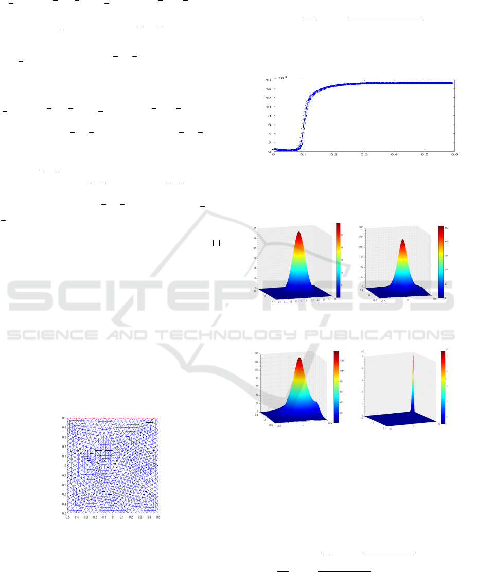
non-admissible grid ﬁgure.1,

Figure 1: The mesh supported in the numerical tests with

h = 0.0471

3.2.1 Test 1

Firstly, we chose the nonsymmetric initial data on a square

(0;5) × (0; 5) and we present the numerical solution of (1)

for different values of t. in this subsection, µ = 1, ξ = 1, the

time step is ∆t = 10

−3

, the number of triangles is 1296 and

the nonsymmetric initial functions is given by

0,1

(x,y) =

2πθ

exp



−

(x − x

)

+ (y − y

)

2θ



, (21)

with the total mass is M = 6π, θ = 10

−2

and x

= y

= 0.1.

Figure 2: Test 1: Time evolution of knk

∞

(Ω)

computed

from the radially non-symmetric initial datum n

0,1

with

M = 6π

Figure 3: Initial datum n

0,1

, t = 0 and t = 0.005

Figure 4: Initial datum n

0,1

, t = 0.015 and t = 1

3.2.2 Test 2

Next, we present the numerical solution of (1) for differ-

ent values of t. in this subsection, µ = 1, ξ = 1, the time

step is ∆t = 10

−3

, the number of triangles is 1296 and the

nonsymmetric initial functions is given by:







0,2

(x,y) =

4π

2πθ

exp



−

(x−x

)

+(y−y

)

2θ



2π

2πθ

exp



−

(x−x

)

+(y−y

)

2θ



(22)

with θ = 10

−2

, x

= y

= 0.1, and x

= y

= −0.2.

Test 2: Cell density computed from nonsymmetric ini-

tial data with M = 6π for different values of t.

The Finite Volume Method Applied to The Patlak-Keller-Segel Chemotaxis Model in a General Mesh

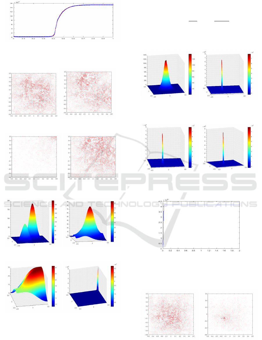
Figure 5: Test 2: Time evolution of knk

∞

(Ω)

computed

from the radially non-symmetric initial datum n

0,2

with the

total mass is M = 6π

Figure 6: Initial datum n

0,2

, t = 0.01 and t = 0.045

Figure 7: Initial datum n

0,2

, t = 0.55 and t = 0.15

Figure 8: Initial datum n

0,1

, t = 0 and t = 0.01.

Figure 9: Initial datum n

0,1

, t = 0.045 and t = 1

3.2.3 Test 3

We now consider the case of radially symmetric initial func-

tions, we present the numerical solution of (1) for different

values of δ. in this subsection, µ = 1, ∆t = 2 × 10

−2

and the

radially symmetric initial function is given by:

0,3

(x,y) =

2πθ

exp



−

+ y

2θ



, (23)

with the mass M = 20π, ξ = 1 and θ = 10

−2

Figure 10: Initial datum n

0,3

, t = 0 and t = 1.5

Figure 11: Initial datum n

0,3

, t = 3 and t = 5

Figure 12: Test 3 : Time evolution of knk

∞

(Ω)

computed

from the radially symmetric initial datum n

0,3

with M =

20π.

Figure 13: Test 3 : Chemical signal concentration computed

from symmetric initial data with M = 20π for t = 0 and

t = 5.5.

ICCSRE 2018 - International Conference of Computer Science and Renewable Energies

4 CONCLUSION

Our numerical results, in the case of radially non-

symmetrical initial data (test 1 and 2), show that the blow-

up occurs at the nearest corner of the point of inoculation

from the 0.1 instant for n

0;1

and 0.4 for n

0;2

, which is com-

patible with cellular dynamics. In the case where the initial

datum is radially symmetrical(test3, the ﬁgures show that

the explosion of the solution of Keller-Segel classical mod-

els occurs at the center of the domain.

REFERENCES

A.Chertock and A.Kurganov (2008). A second-order pos-

itivity preserving central-upwind scheme for chemo-

taxis and haptotaxis models. Numer. Math., 111:169–

205.

A.J.Carrillo, S.Hittmeir, A. u. (2012). Cross diffusion and

nonlinear diffusion preventing blow up in the keller-

segel model. Math. Mod. Meth. Appl. Sci.

AK.Domelevo, P. O. (2005). A ﬁnite volume method for the

laplace equation on almost arbitrary two-dimensional

grids. M2AN Math. Model. Numer. Anal., 39(6):1203–

1249.

A.Marrocco (2003). Numerical simulation of chemotactic

bacteria aggregation via mixed ﬁnite elements. Math.

Mod. Numer. Anal., 4:617–630.

B.Andreianov, F. and F.Hubert (2007). Discrete duality ﬁ-

nite volume schemes for leray-lions type elliptic prob-

lems on general 2d-meshes. Num. Meth. for PDEs,

23:145–195.

Bessemoulin-Chatard, M. and Jungel, A. (2014). A ﬁ-

nite volume scheme for a keller-segel model with ad-

ditional cross-diffusion. IMA Journal of Numerical

Analysis, 34:96–122.

Boyer, F. and Hubert, F. (2008). Finite volume method for

2d linear and nonlinear elliptic problems with discon-

tinuities. SIAM J Numer Anal, 46:3032—-3070.

C. Chainais-Hillairet, S. K. and Mouton, A. (2013).

Study of discrete duality ﬁnite volume schemes

for the peaceman model. SIAM J. Sci. Comput.,

35(6):A2928–A2952.

C.Chainais-Hillairet (2009). Discrete duality ﬁnite vol-

ume schemes for two-dimensional driftdiffusion and

energy-transport models. Internat J Numer Methods

Fluids, 59:239–57.

C.Chainais-Hillairet, S. Krell, A. and Mouton (2015). Con-

vergence analysis of a ddfv scheme for a system de-

scribing miscible ﬂuid ﬂows in porous media. Numer-

ical Methods for Partial Differential Equations, Wiley,

315(3):1098–2426.

Delcourte, S. (2007). D

eveloppement de m

ethodes de vol-

umes ﬁnis pour la m

ecanique des ﬂuides. Ph.d. thesis

(in french), University of Toulouse III, France.

F. Hermeline, S. L. and Omnes, P. (2008). A ﬁnite volume

method for the approximation of maxwell’s equations

in two space dimensions on arbitrary meshes. J Com-

put Phys, 227:9365––9388.

F.Hermeline (2000). A ﬁnite volume method for the approx-

imation of diffusion operators on distorted meshes. J.

Comput. Phys., 160(2):481–499.

G.Chamoun, M. and R.TalhoukF.Filbet (2006). A ﬁnite

volume scheme for the patlak-keller-segel chemotaxis

model. Numer. Math., 104:457–488.

skovec, J. and Schmeiser, C. (2009). Stochastic particle

approximation for measure valued solutions of the 2d

keller-segel system. J. Stat. Phys., 135:133–151.

skovec, J. and Schmeiser, C. (2011). Convergence of

a stochastic particle approximation for measure solu-

tions of the 2d keller-segel system. Commun. Part.

Diff. Eqs., 36:940–960.

Keller, E. and Segel, L. (1970). Initiation of slime mold

aggregation viewed as an instability. J. Theor. Biol.,

26:399–415.

Krell, S. (2011). Stabilized ddfv schemes for stokes prob-

lem with variable viscosity on general 2d meshes.

Numer Methods Partial Differential Eq, pages 1666–

–1706.

Krell, S. (2012). Finite volume method for general multi-

ﬂuid ﬂows governed by the interface stokes problem.

Math Models Methods Appl Sci, 22(5):1150–025.

Krell, S. and Manzini, G. (2012). The discrete duality

ﬁnite volume method for stokes equations on three-

dimensional polyhedral meshes. SIAM J Numer Anal,

50:808—-837.

N.Saito (2007). Conservative upwind ﬁnite-element method

for a simpliﬁed keller-segel system modelling chemo-

taxis. IMA J. Numer. Anal., 27:332–365.

N.Saito (2012). Error analysis of a conservative ﬁnite-

element approximation for the keller-segel model of

chemotaxis. comm. Pure Appl. Anal., 11:339–364.

N.Saito and T.Suzuki (2005). Notes on ﬁnite differ-

ence schemes to a parabolic-elliptic system modelling

chemotaxis. Appl. Math. Comput., 171:72–90.

Patlak, C. (2953). Random walk with persistence and exter-

nal bias. Bull. Math. Biophys, 15:311–338.

R. Strehl, A. Sokolov, D. K. and Turek, S. (2010). A ﬂux-

corrected ﬁnite element method for chemotaxis prob-

lems. Comput. Meth. Appl. Math., 10:219–232.

S.Delcourte, K. D. and P.Omnes (2007). A discrete du-

ality ﬁnite volume approach to hodge decomposi-

tion and div-curl problems on almost arbitrary two-

dimensional meshes. SIAM J Numer Anal, 45:1142—

-1174.

Y. Coudiere, J.-P. V. and Villedieu, P. (1999). Convergence

rate of a ﬁnite volume scheme for a two-dimensional

convection-diffusion problem. M2AN Math. Model.

Numer. Anal., 33:493–516.

Y.Coudi

ere and F.Hubert (2011). A 3d discrete duality ﬁnite

volume method for nonlinear elliptic equations. SIAM

J Sci Comput, 33:1739—-1764.

Y.Coudi

ere and G.Manzini (2010). The discrete duality ﬁ-

nite volume method for convectiondiffusion problems.

SIAM J Sci Comput, 47:4163—-4192.

The Finite Volume Method Applied to The Patlak-Keller-Segel Chemotaxis Model in a General Mesh