
An Overview Graphs Theory and Its Application in Various Scientific
Field
Zahedi
1*
, Suparni
2
, Yenni Suzana
3
and Fachrur Razi
1
1
Department of Mathematics, Universitas Sumatera Utara, Medan, Indonesia
2
State Institute for Islamic Studies Padangsidimpuan, Timbangan, Indonesia
3
State Institute for Islamic Studies Langsa, Langsa, Indonesia
Keywords: Graph Theory, Scheduling, Switching Theory, Physics, Graph Chemistry.
Abstract: As part of mathematics, the use of graphic theory at the present time in various other scientific fields such as
chemistry, physics, engineering and social science, is very widespread. This paper is trying to reveal some
of the uses of graph theory in several fields of science. It is realized that at this time, graph theory has
become one of the topics that attract attention because the models contained in graph theory can be applied
to problems such as transportation, electrical circuit networks, computer science, and many other fields.
Briefly stated that the graph is a representation of a picture of a system that uses two basic elements, namely
points and edges. A point represents a circle and an edge is represented by a line connecting two points.
This paper highlights various views on the application of graphs in the fields of chemistry and physics,
research operations and some general descriptions are presented.
1 INTRODUCTION
As one of the branches of science that is quite old,
graph theory has many applications in various fields
of science. Graph is useful for representing objects
and relationships contained in these objects. Visual
representation of a graph is to declare an object as a
point, circle or dot and the relationship that occurs
between these points is described as a line. An easy
example that can be found in everyday life is a map
of the highway network in a city. As a graph, cities
on the map are expressed by points while lines
connecting the points are edges. In this paper, we
review the notions of graph theory and its use in
several fields by referring to some of the materials
mentioned in the references.
2 GRAPH THEORY
Diagrams that consist of a set of points and lines
connecting certain pairs of points are widely used in
real-world situations. The focus here is about the
two points connected by one line, the way the two
points are connected is not important. It is this
mathematical abstraction that gave rise to the
concept of graphics.
Graph G is sequential triple [V(G), E(G), ∅
]
consisting of non-empty vertices V(G), set E(G),
disjoint from V(G), edges, and ∅
functions events
related to each edge G of the unordered pair of
vertices (not necessarily different) from G. If 𝑒 is the
edge and 𝑢 and 𝑣 are vertices such that PG(e) = 𝑢𝑣,
then 𝑒 is said to join 𝑢 and 𝑣; vertices 𝑢 and 𝑣 are
called ends 𝑒. The following are two examples of
graphs that serve to clarify the situation.
Example 1,
𝐺𝑉
𝐺
,𝐸
𝐺
,∅
, where 𝑉
𝐺
𝑣
,𝑣
,𝑣
,𝑣
,𝑣
and 𝐸
𝐺
𝑒
,𝑒
,𝑒
,𝑒
,𝑒
,𝑒
,𝑒
,𝑒
, and ∅
defined by
∅
𝑒
𝑣
𝑣
, ∅
𝑒
𝑣
𝑣
, ∅
𝑒
𝑣
𝑣
, ∅
𝑒
𝑣
𝑣
∅
𝑒
𝑣
𝑣
, ∅
𝑒
𝑣
𝑣
, ∅
𝑒
𝑣
𝑣
, ∅
𝑒
𝑣
𝑣
Example 2,
𝐻𝑉
𝐻
,𝐸
𝐻
,∅
, where 𝑉
𝐻
𝑢,𝑣,𝑤,𝑥,𝑦, and 𝐸
𝐻
𝑎,𝑏,𝑐,𝑑,𝑒,𝑓,𝑔,ℎ, and
∅
defined by
∅
𝑎
𝑢𝑣, ∅
𝑏
𝑢𝑢, ∅
𝑐
𝑣𝑤, ∅
𝑑
𝑤𝑥
∅
𝑒
𝑣𝑥, ∅
𝑓
𝑤𝑥, ∅
𝑔
𝑢𝑥, ∅
ℎ
𝑥𝑦
326
Zahedi, ., Suparni, ., Suzana, Y. and Razi, F.
An Overview Graphs Theory and Its Application in Various Scientific Field.
DOI: 10.5220/0010181200002775
In Proceedings of the 1st International MIPAnet Conference on Science and Mathematics (IMC-SciMath 2019), pages 326-330
ISBN: 978-989-758-556-2
Copyright
c
2022 by SCITEPRESS – Science and Technology Publications, Lda. All rights reserved

Figure 1: Diagrams of graphs G and H.
Graphs represented graphically help to
understand the properties of the graphs. Each vertex
is represented by a point, and each edge by a line
connecting the points represent the edges. In Figure
1, diagrams G and H are shown in Figure 1. Another
G diagram, is given in Figure 2. The graph diagram
illustrates the relationship between the vertices and
their edges. Note that the two sides in the diagram of
the graph can intersect at points that are not vertices
(for example 𝑒
and 𝑒
of graph G in figure 1).
Figure 2: Another diagrams of G.
Graphs that have diagrams whose edges only
intersect at the edges are called planar, because such
graphs can be represented in simple fields. The
graphic image (3.i) is planar, and the graphic image
(3.ii), on the other hand, is nonplanar. Most of the
definitions and concepts in graph theory are given
by graphical representations. The edges are called
incident with edges, and vice versa. Two vertices
that are adjacent to the same edge are adjacent, as
are the two edges that intersect the common node.
Edges with identical ends are called loops, and edges
with different ends are links. For example, the 𝑒
edge of G (figure 2) is a loop; all other G edges are
links.
Figure 3: Planar and nonplanar graphs.
The graph is limited if the set of vertices and set of
edges is also limited. A graph is called simple if it
does not have a loop and no two links join the same
node pair. Graphic figure 1 is not simple, while the
graphic in figure 3 is simple.
2.1 Graphs in Chemistry and Physics
Graph Theory in Chemistry Graphs are used in
chemistry to model chemical compounds and their
structures. In computational biochemistry, the same
sequence of cell samples must be issued to resolve
conflicts between two sequences. This is modeled in
a graphical form where vertices represent sequences
in the sample. An edge will be drawn between two
vertices if and only if there is a conflict between the
corresponding order. The goal is to remove the
possibility of a node to eliminate all conflicts.
In physics, graphs are used in condensed matter
physics. Usually describes solid state and molecular
systems as a strict binding model. Graph theory is
also widely used in the field of statistical physics.
Statistical physics in the branch of science that deals
with methods of using probability and statistical
theories, and especially mathematical tools for
dealing with large populations and forecasts, in
solving physical problems. The main areas of
statistical physics that use graph theory are statistical
mechanics, particle physics, and statistical analysis
problems and thermodynamic results.
2.2 Graphs in Switching Theory
Ehrenfest (1910), presented a paper on switching
theory where he stated that Boolean algebra could be
applied to automatic telephone exchange. Next
Shannon (1938) introduced a mathematical
formulation of contact network behavior (a
particular type of switching network). Since then,
switching theory has developed very rapidly.
Initially, this was intended for engineers of
communication tools to analyze and synthesize large
scale relay switching networks, such as telephone
exchanges. And, in recent years, the rapid growth of
switching theory was motivated because of its use in
digital computer design. Unlike a signal in a
classical network (say, in a radio receiver), a
switching network signal has only two values -
defined as 0 and 1. A switching network is designed
to process and store the binary signal.
Switching networks can be classified as
combinational networks and / or sequential
networks. Combinational switching networks are
networks that output at a certain time only depend
An Overview Graphs Theory and Its Application in Various Scientific Field
327

on the input at that time. Sequential switching
networks, on the other hand, are those that output at
a particular time are a function of the inputs at that
time and during the entire past history. In other
words, sequential networks have memory, whereas
combinational networks do not. All digital systems,
are built from these two basic types of circuits -
combinations and sequences.
Combinational switching networks can then be
classified as (1) contact networks, or (2) gateway
networks. Here we limit ourselves to the contact
network only.
2.2.1
Contact Networks
Relay contacts (or contacts, for short) can be likened
to ordinary household switches that are used to
control light. This is a two-terminal device that has
two statuses; in the open state where there is no
conductive path between the terminals; and in a
closed state where there is a path that will allow
electric current to flow in both directions. So contact
is a bilateral device. Usually, a contact is represented
by one of the symbols shown in Figure 4 below.
Figure 4: Symbol used to represent a switch or contact.
Contact networks are interconnected networks
where each contact network can be represented by a
graph, where the ends are contacts and the node is
the terminal. For the purpose of writing, a definition
of contact network is given, namely: the contact
network is a directed, connected graph (without its
own loop) where each side has a binary variable 𝑥
associated with it, which can be assumed to have
only two values, 1 or 0 The binary variable 𝑥
specified for a contact is 1 when the contact is
closed and 0 when the contact is open.
The input-ouput behavior of the contact network
is usually expressed in terms of functions,
𝑓
𝑥
,𝑥
,…,𝑥
,
from binary variables. The 𝑓
function is called the
switching function (or Boolean) and is assumed to
have a value of 0 or 1, and where the Boolean
algebra consists of a limited set of 𝑥
,𝑥
,…,𝑥
and
two binary + operations (called Boolean addition)
and . (called Boolean duplication) that meets the
following postulates:
1. Either 𝑥
1 or 𝑥
0
2. For each 𝑥
there is another variable 𝑥
, called
the complementary 𝑥
, so that if 𝑥
0, 𝑥
1,
and if 𝑥
1, 𝑥
0.
3. (a). Sum 𝑥
𝑥
0, 𝑖𝑓 𝑥
𝑥
0,
1, 𝑜𝑡ℎ𝑒𝑟𝑤𝑖𝑠𝑒
(b). Product 𝑥
𝑥
1, 𝑖𝑓 𝑥
𝑥
1,
0, 𝑜𝑡ℎ𝑒𝑟𝑤𝑖𝑠𝑒
with this postulate a number of results can be
derived, which is useful in simplifying the
expression of switching. For example, it can be
easily shown that 𝑥
𝑥
𝑥
𝑥
.
In the contact network, two types of problems
will be found, namely the problem of analysis and
synthesis. Here we will discuss only the problem of
analysis only, where in the analysis given the G
contact network and how to find conditions where
there is an electrical conduction path between a pair
of vertices (𝑣
,𝑣
) in G.
Consider two nodes in the G contact network,
because G is connected, there is one or more paths
between these two nodes. Each path can be
identified by a Boolean product from variables
related to edges in the path. For example, in figure 5,
eight different paths between vertices 𝑎 and 𝑏 are
(𝑥
𝑥
,
𝑥
𝑥
𝑥
,
𝑥
𝑥
𝑥
,
𝑥
𝑥
𝑥
𝑥
,
(𝑥
𝑥
𝑥
,
𝑥
𝑥
𝑥
𝑥
,
𝑥
𝑥
𝑥
,
𝑥
𝑥
𝑥
𝑥
,
(*)
each of these products is called the path product
between nodes 𝑎 and 𝑏 in the contact network of G.
Obviously, the value of the path product is 1 if and
only if each variable in the path product has a value
of 1; if not, it is 0. The value 1 of the product line
implies the existence of an electric conduction path
between 𝑎 and 𝑏 through the appropriate contacts in
the network.
Figure 5: Contact network with six vertices and nine
contacts.
For electrical conduction between two vertices, it
is necessary and sufficient that at least one of the
path products be 1. In other words, the Boolean
number of path products between certain node pairs
(𝑣
,𝑣
) is 1 if and only if terminals 𝑣
and 𝑣
are
electrically connected in the contact network.
Therefore, the number of Boolean line products is
IMC-SciMath 2019 - The International MIPAnet Conference on Science and Mathematics (IMC-SciMath)
328

referred to as the contact network transmission
between two nodes that are determined. For
example, the transmission between vertices 𝑎 and 𝑏
in Figure 5 is
𝐹
𝑥
𝑥
𝑥
𝑥
𝑥
𝑥
𝑥
𝑥
𝑥
𝑥
𝑥
𝑥
𝑥
𝑥
𝑥
𝑥
𝑥
𝑥
𝑥
𝑥
𝑥
𝑥
𝑥
𝑥
𝑥
𝑥
Finding the transmission between the nodes
specified in the given contact network consists of
counting all the paths between the two nodes, and
finding the Boolean number of product lines.
Furthermore, the possibility of simplification based
on Boolean algebraic postulates was also carried out.
For example, in the product lines listed in (*), the
following identities are clear:
𝑥
𝑥
𝑥
𝑥
𝑥
,
𝑥
𝑥
𝑥
𝑥
0,
𝑥
𝑥
𝑥
0,
and
𝑥
𝑥
𝑥
𝑥
0.
Therefore, the switching function between
vertices 𝑎 and 𝑏 in Figure 5 is
𝐹
𝑥
𝑥
𝑥
𝑥
𝑥
𝑥
𝑥
𝑥
𝑥
𝑥
𝑥
𝑥
𝑥
𝑥
Obviously, 𝐹
provides all different conditions
where there is a conductive path between 𝑎 and 𝑏.
2.3 Graphs in Operation
Research - Activity Networks in
Project Planning
One of the most popular network applications in
operations research is the planning and scheduling of
complex projects. A project is divided into many
jobs called activities. Due to technical limitations,
work must be completed before the others start, each
activity also requires the duration or time of the
activity. Several lists of activities in a project,
including a list of direct prerequisites, and duration,
a weighted digraph can be made to describe the
project, as follows: each edge represents the activity,
and the weight represents the duration of the
activity, while the node represents the beginning and
end of the activity. Activity 𝑖,𝑗 cannot start before
all activities 𝑖 have finished. Every event in the
project is a well-defined event in time. Like a
weight, connected graphs describe activities in a
project called the activity network.
Suppose a project consists of six activities P, Q,
R, S, T, and U, with the limitation that P must
precede R and S; Q and S must precede T; and R
must precede U. The duration for activities P, Q, R,
S, T, and U are 5, 7, 6, 4, 15, and 2 days
respectively. This network of project activities is
shown in Figure 6.
Figure 6: Activity network.
Note that network activity must be acyclic; if
not, then there will be an impossible situation where
no activity on the directed circuit can be started.
Also note that the point indicating where the project
starts must have a zero degree, because there are no
activities that precede this point. Likewise, the point
indicating where the project ends must have zero
degrees, because there are no activities after this.
Dummy Activity; in the network activity
example in Figure 6, suppose there is an additional
limitation that activity U cannot begin before Q and
S are completed. This main relationship can be
described as an edge by connecting point 𝑥 to 𝑦
(Fig. 7). This is what is called a dummy activitiy.
Figure 7: Dummy activity in a network.
Dummy activities are important when there are
not enough activities to describe all the relationships
that are prioritized accurately. All puppet activity
has zero duration and is usually displayed in a dotted
line. Two parallel edges (e.g., activities that have the
same direct predecessor and the same direct
successor) can be replaced by one edge, combining
the two activities into one [Fig. 8 (a)]. However, if
activities must be tracked separately, then dummy
activities and dummy events must be created [Fig. 8
(b)]. And, because there is no self-loop in the
activity network, we only have a simple digraph for
the activity network.
An Overview Graphs Theory and Its Application in Various Scientific Field
329
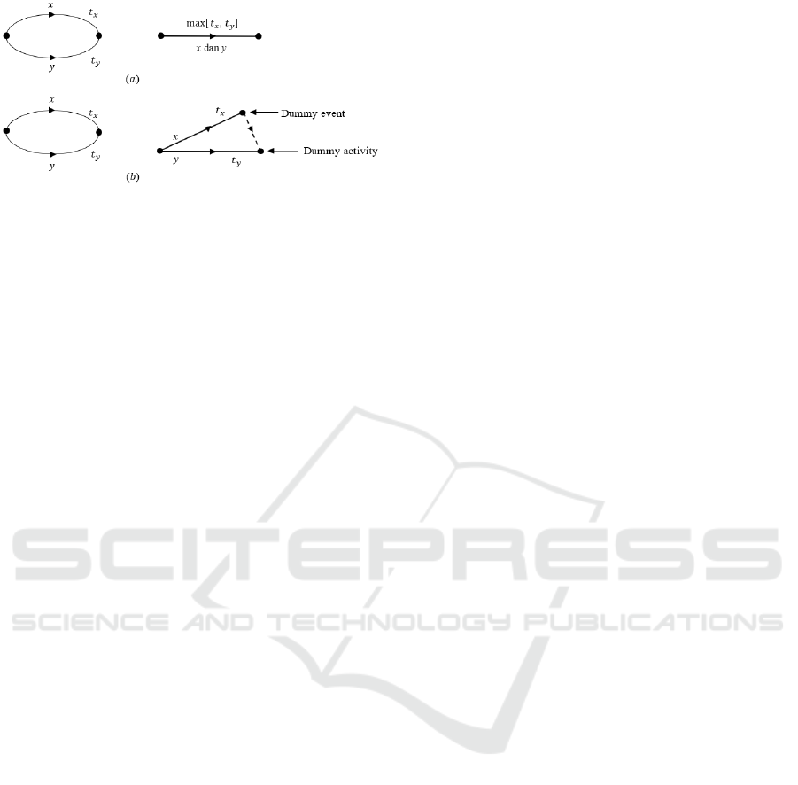
Figure 8: Replacement of parallel edges.
A network of activities can be assumed to have
exactly one node with zero in degrees and exactly
one node with zero outside degrees. If there is more
than one node having zero degrees, someone
arbitrarily chooses one of these for the initial event
and draws the puppet activity from this to the other
node. Vertices with zero degrees are handled
equally.
In short, the activity network is a representation
of two aspects of the project: (1) the priority
relationship between activities, and (2) the time
period. These are connected, weighted, simple,
acyclic digraphs with exactly one zero point in
degrees and exactly one zero point outside the
degree.
3 CONCLUSION
In this paper the author has provided a basic
understanding of graph theory. Understanding is
quite easy to understand and provides a description
of several types of graphs. This paper also explains
where different graphs of graph theory can be used
in various fields of science. In other words, an idea
is given about the use of graphic theory terminology
in its use in various fields of science. Furthermore,
one can understand about this terminology and get
other ideas related to their use in the real world.
REFERENCES
Ehrenfest, P. (1910). Review of L. Coutrat, Algebra of
Logic. J. Russ. Phys. Chem. Soc. Phys. Sec., 42(10),
382–387.
Shannon, C. E. (1938). A Symbolic Analysis of Relay and
Switching Circuits. American Institute of Electrical
Engineers Transactions, 57, 713–723.
IMC-SciMath 2019 - The International MIPAnet Conference on Science and Mathematics (IMC-SciMath)
330
