Supervised Spatial Transformer Networks for Attention Learning in

Fine-grained Action Recognition

Dichao Liu

, Yu Wang

and Jien Kato

3,∗

Graduate School of Informatics, Nagoya University, Nagoya City, Japan

Graduate School of International Development, Nagoya University, Nagoya City, Japan

College of Information Science and Engineering, Ritsumeikan University, Kusatsu City, Japan

Keywords:

Action Recognition, Video Understanding, Attention, Fine-grained, Deep Learning.

Abstract:

We aim to propose more effective attentional regions that can help develop better ﬁne-grained action re-

cognition algorithms. On the basis of the spatial transformer networks’ capability that implements spatial

manipulation inside the networks, we propose an extension model, the Supervised Spatial Transformer Net-

works (SSTNs). This network model can supervise the spatial transformers to capture the regions same as

hard-coded attentional regions of certain scale levels at ﬁrst. Then such supervision can be turned off, and the

network model will adjust the region learning in terms of location and scale. The adjustment is conditioned

to classiﬁcation loss so that it is actually optimized for better recognition results. With this model, we are

able to capture attentional regions of different levels within the networks. To evaluate SSTNs, we construct a

six-stream SSTN model that exploits spatial and temporal information corresponding to three levels (general,

middle and detail). The results show that the deep-learned attentional regions captured by SSTNs outperform

hard-coded attentional regions. Also, the features learned by different streams of SSTNs are complementary

to each other and better result is obtained by fusing the features.

1 INTRODUCTION

Action recognition aims to recognize human actions

from a series of observations, such as video clips and

image sequences. Fine-grained action recognition is a

subclass of action recognition. The term ﬁne-grained

is used similarly in (Rohrbach et al., 2012; Singh

et al., 2016), suggesting that discriminative informa-

tion among different action classes is very subtle. As

shown in Fig. 1, an ordinary action recognition task

may require algorithms to distinguish between com-

pletely different actions. Whereas, ﬁne-grained action

recognition task may require the differentiation of dif-

ferent processes in the same activity. Fine-grained

action recognition is important, useful but also very

difﬁcult. One of the main reasons is that the discri-

minative information among different action classes

is very subtle. Thus, it is difﬁcult to obtain enough

clues from such limited information. It would be pre-

ferable to exploit more comprehensive information

(multi-type and multi-level).

It is quite common for ﬁne-grained action recog-

∗

Corresponding author

(a) (b)

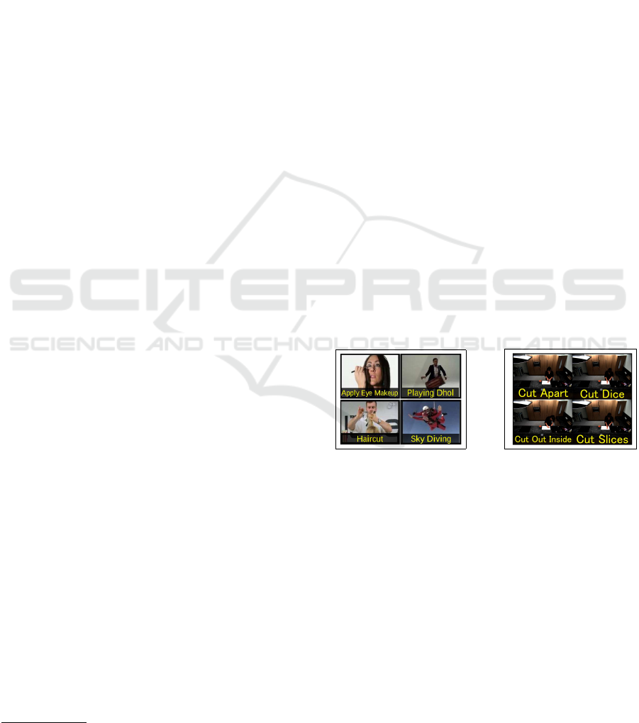
Figure 1: Example of action categories of a general action

recognition task (a) (Soomro et al., 2012) and a ﬁne-grained

action recognition task (b) (Rohrbach et al., 2012). It is

obvious that the differences among different classes in the

ﬁne-grained action recognition task are more subtle.

nition that the discriminative information is only con-

tained in certain parts of a frame while the remaining

parts are redundant. Some studies refer such discri-

minative parts as attentional regions and try to uti-

lize attentional regions rather than full frames to deve-

lop recognition algorithm (Cherian and Gould, 2017;

eron et al., 2015). The utilization of attentional re-

gion is effective because attentional regions can pro-

vide more detailed information and help reduce re-

dundancy. However, the problems of current studies

include the following: (1) they mainly utilize hard-

Liu, D., Wang, Y. and Kato, J.

Supervised Spatial Transformer Networks for Attention Learning in Fine-grained Action Recognition.

DOI: 10.5220/0007257803110318

In Proceedings of the 14th International Joint Conference on Computer Vision, Imaging and Computer Graphics Theory and Applications (VISIGRAPP 2019), pages 311-318

ISBN: 978-989-758-354-4

311

coded approaches (Cherian and Gould, 2017; Ch

eron

et al., 2015), and cannot always obtain the “right”

attentional region (most hard-coded methods assume

attentional regions to be person-centric, which is not

true sometimes); (2) they only explore a certain scale

of regions and ignore the possibly discriminative in-

formation shown in other scales.

Focusing on solving these issues, we turn our

eyes to spatial transformer networks (STNs) (Jader-

berg et al., 2015). STNs allow multiple transforma-

tions on input images to make the transformed ima-

ges to be better recognized. We hope to make use of

this capability to learn attentional regions in an end-

to-end style. By doing so, all factors inﬂuencing the

performance (including how to locate and recognize

the attentional regions) can be optimized together to-

ward the target of better recognition results. However,

the problem is that it is extremely hard to let STNs to

handle all the intended tasks with the only supervision

signal—category labels, especially when we want to

capture more detailed information.

In this work, we propose supervised spatial trans-

former networks (SSTNs), which has a mechanism

named regressive guiding. Regressive guiding lets

spatial transformers to capture the regions same as

hard-coded attentional regions of certain scales by

regression. With SSTNs, we can ﬁrst guide the

networks to capture attentional regions (rather than

performing other transformations) of intended sca-

les. Then we turn off regressive guiding and let the

networks to adjust region localization by themselves

(with only categorical information). Finally, the deep-

learned attentional regions from SSTNs will focus on

more meaningful and discriminative parts.

To throughout evaluate the attentional regions

captured by SSTNs, we built SSTNs of six streams,

which captures two types of information (RGB fra-

mes and optical ﬂows) in three levels(detail, middle

and general). Those SSTNs are then proved to be

more effective than the STNs in the same cases for

capturing deep-learned attentional regions. Then for

comparison, we also train six streams of CNNs on the

relevant hard-coded attentional regions (RGB frames

and optical ﬂows from detail to general level). We

then compare the recognition performance between

those SSTNs and CNNs. We ﬁrst use this SSTNs/

CNNs to extract deep features for every frame in a

video clip and then aggregate those frame-level fea-

tures to be video-level descriptors by temporal cor-

relation pooling (TCP) (Cherian and Gould, 2017).

The results demonstrate that the deep-learned attenti-

onal regions perform better than the hard-coded ones.

The attentional regions captured by SSTNs are more

action-centric rather than person-centric as the hard-

coded ones. The results also show that the six SSTNs

streams are complementary to each other, and fusing

them can bring better performance.

2 RELATED WORKS

Recently, the studies on action recognition has de-

veloped a lot from traditional shallow approaches to

newly-developed deep approaches. Shallow methods

derives the properties using the information contained

in the videos themselves (Wang et al., 2011; Wang

et al., 2013; Dalal et al., 2006), and have been pro-

ved to be effective. However, the deep methods, es-

pecially the CNNs, further boost the performance of

action recognition (Le et al., 2011; Wang et al., 2016;

Simonyan and Zisserman, 2014a; Wang et al., 2015;

Feichtenhofer et al., 2016), such as the two-stream

models (Wang et al., 2016; Simonyan and Zisserman,

2014a; Wang et al., 2015; Feichtenhofer et al., 2016).

In two-stream models, one of the streams is fed with

RGB frames to capture spatial information. The other

is fed with optical ﬂows to capture motion informa-

tion. Our work is also inspired by two-stream models.

We exploit both spatial and temporal information.

In ﬁne-grained visual recognition, discriminative

clues are always very subtle. For avoiding redun-

dancy, some works make effort to ﬁnd and learn the

regions of interest rather than the entire scenes. Such

effort can be divided into two types, namely hard-

coded attention and deep-learned attention. Hard-

coded attention generally selects the attentional re-

gions before learning them. The selection is always

implemented by solving a certain statistical problem,

which always strongly relays on human’s expert kno-

wledges (Ba et al., 2015). The selected regions can

then be learned by recognition algorithms. Deep-

learned attention is generally implemented with cer-

tain learnable mechanisms designed for attention le-

arning, which can be embedded within the networks.

Such attention-learning models can be trained toget-

her with the recognition networks by standard back-

propagation. For example, (Li et al., 2018) generates

video saliency maps for locating attentions with the

feature maps from VideoLSTM, which is able to si-

multaneously exploit multiple video information (ap-

pearance, motion and attention). By doing so, (Li

et al., 2018) brings relevant spatial-temporal locations

for video-based attentional regions. Another example

is (Sharma et al., 2015), which takes the 7 ×7×1024-

D feature cubes from CNNs as the inputs of their

LSTM-based attention model.

Among those works, our work is mainly inspi-

red by (Jaderberg et al., 2015). For recognizing ﬁne-

VISAPP 2019 - 14th International Conference on Computer Vision Theory and Applications

312

grained image, (Jaderberg et al., 2015) proposes the

Spatial Transformer, which can apply multiple trans-

formations on the inputs. The transformation could

possibly make the transformed images to be attenti-

onal regions of the input images. However, for the

video-based case, as we observe that (Jaderberg et al.,

2015) suffers from the mentioned problem, we pro-

pose a supervised variant of (Jaderberg et al., 2015).

The supervising signals are computed from hard-

coded attentional regions obtained by a motion-heavy

strategy that is similar to (Singh et al., 2016; Cherian

and Gould, 2017). The work of (Chen et al., 2016) is

also a supervised variant of (Jaderberg et al., 2015).

However, our work is still very different from (Chen

et al., 2016), because: (1)Beside the categorical la-

bels, (Chen et al., 2016) requires another ground truth,

namely the facial landmarks, which is quite unique for

face detection. However, we only use categorical la-

bels as ground truth. Motion-heavy regions are used

for supervision, which apparently cannot be regarded

as ground truth. (2) (Chen et al., 2016) supervises the

spatial transformer via an FC layer. However, with re-

gressive guiding, we directly supervise by the inten-

ded initial transformation parameters. Our methods

is more direct and easier to theoretically explain as

there is no “black box” (i.e., the FC layer) between

the supervising target and signal. (3) In (Chen et al.,

2016), the supervision module works all the time. In

our work, after the supervision, the supervision mo-

dule is “turned off ”. Thus, in the latter stage, our

work is optimized only towards the target of better

recognition without being inﬂuenced by manual sig-

nals. (4) By different initialization, our approach is

able to obtain attentional information of multiple sca-

les, which provide complementary information.

Above-mentioned works are mainly about obtai-

ning the information of single frames. There are

some studies focusing on pooling schemes that aggre-

gate frame-level features into a video-level represen-

tation. Temporal correlation pooling (TCP) (Cherian

and Gould, 2017), for example, is a temporal pool-

ing scheme based on second-order pooling. Besides,

(Cherian et al., 2017b) also tries to analyze higher-

order statistics among frame-level features.

3 APPROACH

3.1 STNs in Attention Learning

STNs are initially designed for image alignment. As

shown in Fig. 2, STNs can be roughly divided into

two parts: the localization network and the recogni-

tion network. Given an input image I

, the localiza-

tion network can learn a set of transformation para-

meters θ = f

loc

), where f

loc

denotes the function

of the localization network. Thereafter a sampler T

obtains the transformed image I

= T (θ, I

), and I

will be the input of the recognition network. The

whole structure can be optimized together: thus, the

transformation applied on I

will make I

better re-

cognized by the recognition network. To obtain I

T utilizes a parameterized sampling grid. For exam-

ple, assume T (θ, I

) applies afﬁne transformation on

. Thereafter θ =





is an afﬁne trans-

formation matrix. Let G be a regular grid, and I

deﬁned on it. (x

, y

) are the target coordinates of the

pixel of G. (x

, y

) are the sampling coordinates in

. The transformation is

















(1)

In addition to afﬁne, STNs also allow other trans-

formations, such as cropping, rotation and scaling. In

our work, we hope the spatial transformers to cap-

ture the attentional regions. However, it is hard to

make the localization network automatically “know”

our intention. The networks can hardly automatically

perform the cropping of right scale, rather than other

transformations, when only categorical information is

provided. Furthermore, in many cases, the images

obtained from localization networks are severely dis-

torted. We refer this problem as “Distortion Effect”.

Figure 2: Illustration of STNs. The localization net can

learn a set of transformation parameters θ from input image

. With θ, sampler T transfers I

to I

, which will be the

input of the recognition network.

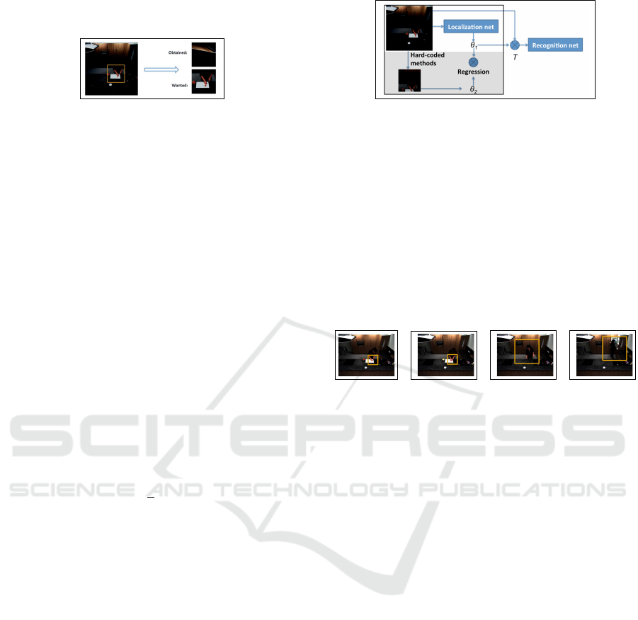
Distortion Effect: As shown in Fig. 3, the pur-

pose of using STNs is to learn the attentional regi-

ons from input frames. However, what we actually

obtain from STNs are distorted images that cannot be

well recognized by the recognition network. This is

because initial parameters of spatial transformer mo-

dules are random. Therefore, at the beginning, the

transformation applied on video frames is meaning-

less. In many cases, especially when we want more

detailed information, however STNs are trained, they

still obtain only distorted images. It is because in such

Supervised Spatial Transformer Networks for Attention Learning in Fine-grained Action Recognition

313

cases, STNs can hardly be optimized with only classi-

ﬁcation loss propagated from a recognition network.

Figure 3: Illustration of “Distortion Effect”. We hope to

obtain attentional regions, but only obtained distorted ima-

ges.

3.2 SSTNs

To solve the problem of “Distortion Effect” as well

as capture multi-level attentional regions, we propose

SSTNs, which initialize the localization network with

hard-coded attentional region by regressive guiding.

Then, regressive guiding is turned off and localization

network is jointly trained with recognition network.

Hard-coded Attentional Region Generation: We

utilize optical ﬂows to locate hard-coded attentional

region. p represents a certain frame, whose size is

w × h and w is the long side. O = {o

, o

, ..., o

} are

l optical ﬂows around p. We ﬁrst compute the mo-

tion value map M by (2). In (2), α and β denote the

spatial location of pixels. We then use a window of

size v × v(w > h > v) to traverse M. Thereafter, we

use the window which has the most motion value to

bound the hard-coded attentional region.

α,β

∑

i=1

i,α,β

(2)

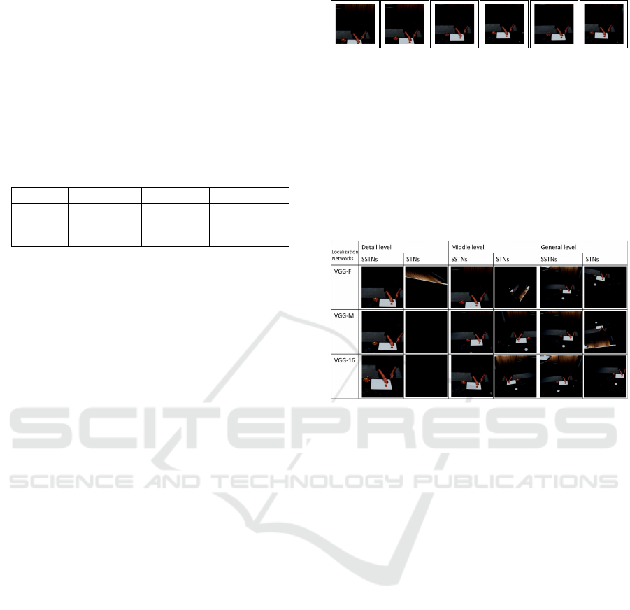
Regressive Guiding: As shown in Fig. 4, we initia-

lize the localization network by regression. Let I be

the input image. θ

= f

loc

(I), is the transformation

parameters directly computed from the input image

by a localization network. θ

is also a set of transfor-

mation parameters and T (θ

, I) is equal to the hard-

coded attentional region R

. θ

can be computed be-

forehand according to the knowledge in Section 3.1

(θ

is actually a rotation matrix, and both R

and I are

already known). During regressive training, θ

is the

regressive objective. The network is trained by redu-

cing the l

loss incurred by θ

against θ

. After the

training, given input images, the localization network

will output approximate R

We then fuse the initialized localization network

with the recognition network and train them toget-

her (joint training). During the joint training, the net-

works will gradually locate from R

to deep-learned

attentional region R

, which is more discriminative.

Figure 4: Illustration of the SSTNs. The parts in the black

frame box are the parts that implement regressive guiding.

Inside the black frame box, except the shaded parts, the rest

parts are actually existing parts of STNs. During regres-

sive guiding, the parts outside of the black frame box are

turned off (truncated). After regressive guiding, for further

adjusting the attentional regions, the shaded parts are tur-

ned off and all the other parts are turned on (linked up). In

this ﬁgure, θ

is the transformation parameters outputted by

localization network. θ

is the transformation parameters,

with which the sampler T will output the same region as

hard-coded attentional regions. During regressive guiding,

we use θ

as regression target and train the parts in the black

frame box by minimizing the l

loss between θ

and θ

(a) (b) (c) (d)

Figure 5: When distinguishing between “cut outside” (a)

and “cut slices” (b), it is obvious that discriminative infor-

mation is mainly contained in detailed region. However, in

some other cases, such as distinguishing between “take out

from drawer” (c) and “take out from fridge” (d), more ge-

neral information, such as the position of human (whether

the person is closer to the fridge or drawer), is also impor-

tant

3.3 Multi-stream SSTNs

When smaller attentional regions can provide more

detailed information, sometimes more general infor-

mation is also crucial (Fig. 5). To provide all-round

information, we apply three levels of attentional regi-

ons, namely detail level, middle level and general le-

vel. Multi-stream networks are developed to learn two

types of information (RGB frames and optical ﬂows)

for each of the three levels of attentional regions (ge-

neral, middle and detail). Thus our whole framework

has totally six streams of SSTNs (Fig. 6).

To obtain different levels of attentional regions,

we ﬁrst resize the original frame I

ori

× h

ori

) to

, whose size is w

× h

ori

, w

are the long si-

des). We then randomly crop a h

×h

part I

crop

from

. Then we need to obtain the deep-learned atten-

tional region R

with the localization network f

loc

()

and the cropped frame I

crop

. In this work, localization

network and recognition network require the inputs

of the same and deﬁnite size (let it be h

× h

. e.g.,

VISAPP 2019 - 14th International Conference on Computer Vision Theory and Applications

314

224 × 224). Thus, we ﬁrst downscale (e.g., spatial

pooling or image resizing) I

crop

to I

crop

whose size is

× h

. Then we can compute the transformation

parameter θ = f

loc

crop

). Then R

can be obtained

by R

= T (θ, I

crop

). We set up T to output R

to be

the size of h

× h

. θ is initialized by regressive gui-

ding beforehand to make T to capture a region of a

certain scale from I

crop

. It is obvious that the scale is

determined by the sizes of I

crop

and R

. Since the size

of R

is deﬁnite, the scale is actually determined by

. Thus, if we set w

and h

to be larger, R

will be

more detailed; otherwise, it will be more general.

Therefore, we can initialize multi-level localiza-

tion networks with multi-size I

crop

and the correspon-

ding R

. Then the attentional regions can be ﬁne-

tuned according to the classiﬁcation loss.

3.4 Temporal Correlation Pooling

By far, what we introduced is about exploring infor-

mation from single frames (or a sequence of optical

ﬂows around a single frame). In this section, we intro-

duce how we aggregate the information from different

frames of a video clip.

For this, we mainly apply TCP (Cherian and

Gould, 2017), which is a second-order pooling

scheme for pooling a temporal sequence of features.

Let V = {v

, v

, ..., v

} be feature vectors com-

puted from frames P = {p

, p

, ..., p

, ... p

} of a vi-

deo clip C. v

= {κ

, κ

, ..., κ

} is a m-

dimensional feature vector of the n

frame in C. Tra-

jectory is deﬁned as t

= {κ

, κ

, ..., κ

}, j ∈

{1, 2, ..., m}. TCP summarizes the similarities bet-

ween each pair of trajectories in a symmetric positive

deﬁnite matrix S ∈ R

m×m

. For example, the value of

the i

row and j

column in S could be given by :

i, j

= E

dis

) (3)

where E

dis

denotes Euclidean distance. In our work,

after training the networks, we extract frame-level

deep features and use TCP to pool those features to

obtain video-level features, as shown in Fig. 6.

Figure 6: Structure of the proposed approach. Totally six

streams learns multi-level spatial-temporal features, which

is then pooled and fused into video-level representation.

4 EVALUATION

The evaluation can be mainly divided into two parts.

The ﬁrst part is to conﬁrm that SSTNs are ef-

fective for capturing deep-learned attentional regions

(Section 4.2). We evaluate multi-level SSTNs and

STNs with localization networks of different parame-

ter sizes. By single-frame validation, we conﬁrm that

SSTNs outperform STNs in every scale. The second

part is to conﬁrm the improvement brought by propo-

sed approach over traditional hard-coded approaches

by all-frame validation (Section 4.3).

4.1 Dataset and Implementation Details

Dataset: To evaluate our approach, we use the MPII

Cooking Activities Dataset (Rohrbach et al., 2012),

which is a dataset of cooking activities. The dataset

contains 5609 clips, 3748 of which are labeled as one

the of 64 distinct cooking activities, and the remaining

1861 are labeled as background activity.

Networks: We utilize the VGG-16 model (Simonyan

and Zisserman, 2014b) for all the recognition net-

works . For localization networks, we utilize VGG-

F, VGG-M (Chatﬁeld et al., 2014) and VGG-16. We

set the batch size as 128 with sub-batch strategy. We

set the dropout ratio as 0.85 for the spatial recognition

networks and 0.5 for the temporal ones. The dropout

ratio of all localization networks are set as 0.5. We

ﬁrst train the localization network by regressive gui-

ding and pre-train the recognition networks by rand-

omly cropping on I

. At this stage, we set the lear-

ning rate as 10

−3

for localization networks and 10

−4

for recognition networks. We then fuse localization

and recognition networks for joint training. At this

stage, we set the learning rate as 10

−6

for localization

networks and 10

−5

for recognition networks. When

training CNNs directly on hard-coded attentional re-

gions, the learning rate is set as 10

−4

at ﬁrst and then

−5

when training status saturates.

Attentional Region: The original size of frames in

the dataset is 1624 × 1224. Table 1 shows the sizes of

, I

crop

and I

crop

/ R

for different levels. Regar-

ding the downscaling strategy for obtaining I

crop

from

crop

, we utilize resizing for general level. For middle

and detail level, we respectively add 2× and 4× max

pooling layers before the localization networks.

Temporal Pooling: After completing the training of

networks, we extract FC6 features for every frame in

video clips. We then use TCP to pool the frame-level

features to a video-level representation. However, dif-

fering from (Cherian and Gould, 2017), we use PCA

to reduce the dimension of FC6 features (4096-d to

256-d), rather than block-diagonal kernelized correla-

Supervised Spatial Transformer Networks for Attention Learning in Fine-grained Action Recognition

315

tion pooling (BKCP).

Multi-stream Fusion: As mentioned before, our ﬁ-

nal structure consists of 6 streams. Each stream is

trained separately. Therefore, we obtain six types of

video-level representations by six streams. For each

of the three levels (detail, middle and general), we

concatenate spatial and temporal video-level repre-

sentations and use them to train a linear SVM. Pre-

diction scores from the three SVMs are applied with

average fusion to be the ﬁnal prediction scores.

Table 1: Size conﬁguration for different levels

Level I

crop

/ R

Detail 1189 × 896 896 × 896 224 × 224

Middle 594 × 448 448 × 448 224 × 224

General 340 × 256 256 × 256 224 × 224

4.2 Comparison between SSTNs/ STNs

In this section, we evaluate the classiﬁcation perfor-

mance of SSTNs by comparing SSTNs with STNs re-

spectively in detail, middle and general levels. For

each level, we respectively utilize VGG-F, VGG-M

and VGG-16 to act as the localization networks of

SSTNs and STNs. For controlling variables, all the

recognition networks are VGG-16. The three dif-

ferent kinds of localization networks are similar in

structures, but different in the depth of layers, the

pixel stride of certain convolutional layers and con-

sequently the size of total parameters. The parameter

sizes of VGG-F, VGG-M and VGG-16 are respecti-

vely about 227M, 384M and 515M.

The main objective of this section is to evaluate

whether and to what extend SSTNs can outperform

STNs in different cases. Then, we can decide how we

can propose more effective deep-learned attentional

regions based on the evaluation results. For speed-

precision trade-off, in this section, we evaluate the

one-vs-all accuracies of different SSTNs and STNs

by randomly selecting a single frame per video, rat-

her than aggregating the information learned from all

the frames of each video. The evaluation results are

shown in Table 2. We also show the regions captured

by different STNs and SSTNs in Fig. 8.

It can be observed that:

Detail Level. The improvements brought by SSTNs

in this level are most noticeable. Whereas the accu-

racy of STNs are very low, suggesting STNs can

hardly capture the information of this level. In con-

trast, for SSTNs, when utilizing the localization net-

works of same size, the accuracies in detail level are

the highest. Moreover, for STNs, the larger the locali-

zation network is, the harder it is to optimize. Conver-

sely, the SSTNs with more parameters in localization

networks have better results.

(a) (b) (c) (d) (e) (f)

Figure 7: (a-f) show the middle-level attentional regions

captured by SSTNs during the joint training. (a) is the at-

tentional region captured by the SSTN that is just initialized

by regressive guiding. Thus, (a) can be regarded to be equal

to the hard-coded attentional region. (f) is the attentional

region captured by the SSTN when the joint training is ﬁ-

nished. (b-e) are attentional regions captured by SSTNs in

different stages between (a) and (f). It can be seen that from

(a) to (f), SSTNs gradually focus on more informative regi-

ons with the action-happening region coming to the center

of the scene (from person-centric to action-centric).

Figure 8: Illustration of the deep-learned attentional regi-

ons captured by different SSTNs and STNs after the trai-

ning. Overall, all STNs suffer from Distortion Effect to

some extend. Especially in detail level, “Distortion Effect”

is so severe that STNs can get almost none detail-level in-

formation. On the contrary, SSTNs can capture attentio-

nal regions as intended without being affected by “Distor-

tion Effect”. Among different levels, the detail-level SSTN

mainly captures the objects concerned with the action, such

as hands and knife. The general-level SSTN preserves much

background information and the middle-level SSTN captu-

res the information between the detail and general SSTNs.

Moreover, for SSTNs, in the attentional regions captured by

the larger localization networks, the action-happening place

is more central in the captured scenes.

Middle Level. SSTNs outperform STNs. For

SSTNs, larger localization networks bring better re-

sults. Whereas for STNs, the one using VGG-16 per-

forms worst.

General Level. SSTNs outperform STNs. For

SSTNs, the localization networks with more parame-

ters get better results. However, for STNs, the ones

that use VGG-16 and VGG-F as localization networks

have similar performance while the one using VGG-

M performs much worse than them.

To sum up, SSTNs improve the performance over

STNs. Among the three levels, detail-level infor-

mation is most effective but only can be explored

by SSTNs. Larger localization networks should be

more capable but only SSTNs can release the poten-

VISAPP 2019 - 14th International Conference on Computer Vision Theory and Applications

316

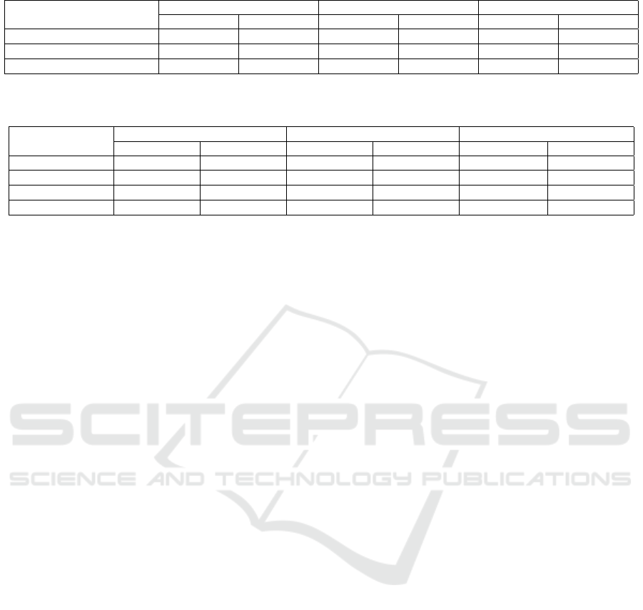
Table 2: Comparison on single-frame classiﬁcation performance (one-vs-all accuracy) of SSTNs and STNs

Localization networks

Detail level Middle level General level

STNs SSTNs STNs SSTNs STNs SSTNs

VGG-F 10.67% 29.91% 25.53% 28.68% 29.02% 29.41%

VGG-M 7.97% 31.09% 28.68% 29.91% 23.95% 29.46%

VGG-16 6.39% 32.32% 28.38% 30.64% 29.1% 30.1%

Table 3: All-frame classiﬁcation performance (mAP) comparison between hard-coded (R

) and deep-learned (R

) attentional

regions. “S + T” denotes concatenating spatial and temporal video-level representations.

Spatial Temporal S + T

General 41.73% 38.98% 54.78% 54.18% 56.51% 56.68%

Middle 50.92% 50.53% 56.23% 52.87% 61.02% 58.96%

Detail 52.75% 51.4% 59.07% 49.18% 62.01% 58.27%

Late fusion 56.08% 55.06% 60.83% 57.38% 63.16% 60.09%

tial. Thus, in the next section, we utilize SSTNs with

VGG-16 as localization network to capture multi-

level deep-learned attentional regions.

4.3 Comparison between Hard-coded/

Deep-learned Attentional Regions

Table 3 shows the mAP results of recognition net-

works trained on hard-coded (R

) and deep-learned

) attentional regions. It is obvious that R

per-

forms better than R

in all aspects. In the detail level

of temporal stream, performance is improved mostly

from R

to R

. Also, it can be inferred that detail-level

performs better than middle-level R

, and middle-

level R

performs better than general-level R

Moreover, the three levels of features are comple-

mentary to each other. With late fusion, the perfor-

mance can be further improved. Fig. 7 uses middle-

level attentional regions as an example, showing the

attentional regions captured by SSTNs during the dif-

ferent stages of joint training. The ﬁgure illustrates in

the manner in which SSTNs gradually move the focus

from person-centric to action-centric.

Regarding the state-of-art works (Cherian et al.,

2017a; Cherian and Gould, 2018) on this dataset,

rather than learning more informative features from

each frame, they focus on the pooling schemes for

aggregating information from different frames, which

is not the point we focus on at all. Besides, those

state-of-art performances are achieved by combining

with shallow features. However, in this paper, for

comparing the performance between hard-coded and

deep-learned attentional regions, our evaluation sim-

ply uses a simple version of TCP and does not inte-

grate with shallow features. Therefore, in fact, it is

quite not meaningful to compare our work with the

state-of-art works. However, since those state-of-art

works are about temporal pooling, they are actually

complementary with our work. Since our work intro-

duces an effective approach for capturing more dis-

criminative deep-learned attentional regions, we sup-

pose the recognition results may be further improved

by aggregating the frame-level features obtained from

our approaches by those pooling methods.

5 CONCLUSIONS

We introduce a new extension model of STNs, the

SSTNs. With the mechanism of regressive guiding,

SSTNs are able to let the spatial transformers to un-

derstand their “mission”. Regressive guiding super-

vises spatial transformers to capture multi-level atten-

tional regions according to the hard-coded attentional

regions at ﬁrst. Then regressive guiding is turned off

and the model is able to adjust to capture more ef-

fective regions. Also, with regressive guiding, spatial

transformers do not suffer from “Distortion Effect”.

It is clear that, the spatial transformers supervised by

the mechanism perform the operation of region cap-

turing while the spatial transformers without the me-

chanism tend to get distorted images. Furthermore,

the SSTNs with larger localization networks capture

more effective attentional regions. The deep-learned

attentional regions help SSTNs to gain better recog-

nition results than the CNNs trained on hard-coded

attentional regions. Moreover, the streams of multi-

stream SSTNs are complementary to each other. The

fusion of them brings better results.

ACKNOWLEDGEMENT

This work is supported by the JSPS Grant-in-Aid for

Young Scientists (B) (No.17K12714), the JST Center

of Innovation Program and PhD Program Toryumon.

Supervised Spatial Transformer Networks for Attention Learning in Fine-grained Action Recognition

317

REFERENCES

Ba, J., Salakhutdinov, R. R., Grosse, R. B., and Frey, B. J.

(2015). Learning wake-sleep recurrent attention mo-

dels. In Advances in Neural Information Processing

Systems, pages 2593–2601.

Chatﬁeld, K., Simonyan, K., Vedaldi, A., and Zisserman,

A. (2014). Return of the devil in the details: Delving

deep into convolutional nets. In British Machine Vi-

sion Conference.

Chen, D., Hua, G., and Wen, F. (2016). Supervised trans-

former network for efﬁcient face detection. In Euro-

pean Conference on Computer Vision, pages 122–138.

Springer.

Cherian, A., Fernando, B., Harandi, M., and Gould, S.

(2017a). Generalized rank pooling for activity recog-

nition. arXiv preprint arXiv, 170402112.

Cherian, A. and Gould, S. (2017). Second-order tempo-

ral pooling for action recognition. arXiv preprint

arXiv:1704.06925.

Cherian, A. and Gould, S. (2018). Second-order temporal

pooling for action recognition. International Journal

of Computer Vision.

Cherian, A., Koniusz, P., and Gould, S. (2017b). Higher-

order pooling of CNN features via kernel linearization

for action recognition. CoRR, abs/1701.05432.

eron, G., Laptev, I., and Schmid, C. (2015). P-cnn: Pose-

based cnn features for action recognition. In Procee-

dings of the IEEE international conference on compu-

ter vision, pages 3218–3226.

Dalal, N., Triggs, B., and Schmid, C. (2006). Human de-

tection using oriented histograms of ﬂow and appea-

rance. In European conference on computer vision,

pages 428–441. Springer.

Feichtenhofer, C., Pinz, A., and Zisserman, A. (2016). Con-

volutional two-stream network fusion for video action

recognition. In Proceedings of the IEEE Conference

on Computer Vision and Pattern Recognition, pages

1933–1941.

Jaderberg, M., Simonyan, K., Zisserman, A., et al. (2015).

Spatial transformer networks. In Advances in Neural

Information Processing Systems, pages 2017–2025.

Le, Q. V., Zou, W. Y., Yeung, S. Y., and Ng, A. Y. (2011).

Learning hierarchical invariant spatio-temporal featu-

res for action recognition with independent subspace

analysis. In Computer Vision and Pattern Recogni-

tion (CVPR), 2011 IEEE Conference on, pages 3361–

3368. IEEE.

Li, Z., Gavrilyuk, K., Gavves, E., Jain, M., and Snoek, C. G.

(2018). Videolstm convolves, attends and ﬂows for

action recognition. Computer Vision and Image Un-

derstanding, 166:41–50.

Rohrbach, M., Amin, S., Andriluka, M., and Schiele, B.

(2012). A database for ﬁne grained activity detection

of cooking activities. In Computer Vision and Pattern

Recognition (CVPR), 2012 IEEE Conference on, pa-

ges 1194–1201. IEEE.

Sharma, S., Kiros, R., and Salakhutdinov, R. (2015). Action

recognition using visual attention. arXiv preprint

arXiv:1511.04119.

Simonyan, K. and Zisserman, A. (2014a). Two-stream

convolutional networks for action recognition in vi-

deos. In Advances in neural information processing

systems, pages 568–576.

Simonyan, K. and Zisserman, A. (2014b). Very deep con-

volutional networks for large-scale image recognition.

arXiv preprint arXiv:1409.1556.

Singh, B., Marks, T. K., Jones, M., Tuzel, O., and Shao, M.

(2016). A multi-stream bi-directional recurrent neural

network for ﬁne-grained action detection. In Procee-

dings of the IEEE Conference on Computer Vision and

Pattern Recognition, pages 1961–1970.

Soomro, K., Zamir, A. R., and Shah, M. (2012). Ucf101:

A dataset of 101 human actions classes from videos in

the wild. arXiv preprint arXiv:1212.0402.

Wang, H., Kl

aser, A., Schmid, C., and Liu, C.-L. (2011).

Action recognition by dense trajectories. In Computer

Vision and Pattern Recognition (CVPR), 2011 IEEE

Conference on, pages 3169–3176. IEEE.

Wang, H., Kl

aser, A., Schmid, C., and Liu, C.-L. (2013).

Dense trajectories and motion boundary descriptors

for action recognition. International journal of com-

puter vision, 103(1):60–79.

Wang, L., Qiao, Y., and Tang, X. (2015). Action recog-

nition with trajectory-pooled deep-convolutional des-

criptors. In Proceedings of the IEEE Conference

on Computer Vision and Pattern Recognition, pages

4305–4314.

Wang, Y., Song, J., Wang, L., Van Gool, L., and Hilliges,

O. (2016). Two-stream sr-cnns for action recognition

in videos. In BMVC.

VISAPP 2019 - 14th International Conference on Computer Vision Theory and Applications

318