Vehicle Activity Recognition using Mapped QTC Trajectories

Alaa AlZoubi

and David Nam

School of Computing, The University of Buckingham, Buckingham, U.K.

Centre for Electronic Warfare, Information and Cyber, Cranﬁeld University, Defence Academy of the UK, U.K.

Keywords:

Vehicle Activity Recognition, Qualitative Trajectory Calculus, Trajectory Texture, Transfer Learning, Deep

Convolutional Neural Networks.

Abstract:

The automated analysis of interacting objects or vehicles has many uses, including autonomous driving and

security surveillance. In this paper we present a novel method for vehicle activity recognition using Deep

Convolutional Neural Network (DCNN). We use Qualitative Trajectory Calculus (QTC) to represent the re-

lative motion between pair of vehicles, and encode their interactions as a trajectory of QTC states. We then

use one-hot vectors to map the trajectory into 2D matrix which conserves the essential position information

of each QTC state in the sequence. Speciﬁcally, we project QTC sequences into a two dimensional image

texture, and subsequently our method adapt layers trained on the ImageNet dataset and transfer this know-

ledge to the activity recognition task. We have evaluated our method using two different datasets, and shown

that it out-performs state-of-the-art methods, achieving an error rate of no more than 1.16%. Our motivation

originates from an interest in automated analysis of vehicle movement for the collision avoidance application,

and we present a dataset of vehicle-obstacle interaction, collected from simulator-based experiments.

1 INTRODUCTION

The vehicle activity recognition task aims to iden-

tify the actions of one or more vehicles from a se-

quence of observations. The pair-wise interaction be-

tween vehicle-vehicle or vehicle-obstacle is the buil-

ding block of large group interactions. In dynamic

trafﬁc a vehicle will share the same roads with dif-

ferent objects (e.g. vehicles or obstacles), on which

unexpected interactions can occur anytime and any-

where. Quite often vehicular collisions are a result

of a lack of situational awareness, and not being able

to identify situations before they become dangerous.

Therefore, understanding the relative interaction bet-

ween the vehicle and it is surrounding is crucial for re-

cognizing the behavior that the vehicle is in (or about

to enter) and to avoid any potential collisions (Ohn-

Bar and Trivedi, 2016).

Previous research concerned with vehicle activity

analysis has been mainly focused on quantitative met-

hods which use sequences of real-valued features (tra-

jectories) (Xu et al., 2017; Khosroshahi et al., 2016;

Lin et al., 2013; Lin et al., 2010; Ni et al., 2009;

Zhou et al., 2008). However, increasing attention has

been given to the use of qualitative methods, which

use symbolic rather than real-value features, with ap-

plications such as, vehicle interaction and human be-

havior analysis (AlZoubi et al., 2017), and human-

robot interaction (Hanheide et al., 2012). Qualita-

tive methods have shown better performance for vehi-

cles activity analysis (AlZoubi et al., 2017). There

are several motivations for using qualitative methods

such as: qualitative representations are typically more

compact and computationally efﬁcient than quantita-

tive methods, and humans naturally communicate and

reason in qualitative ways rather than by using quanti-

tative measurements, particularly when describing in-

teractions and behaviors (Dodge et al., 2012).

In the context of activity recognition a few previ-

ous studies made their efforts on encoding the trajec-

tory of moving object in a compact and powerful re-

presentation (e.g. two dimensional matrix (Lin et al.,

2013) or trajectory texture image (Shi et al., 2015).

These features were used to train the classiﬁer for the

activity recognition task. These methods have shown

to be successful in different application domains va-

ries between human activity recognition (Shi et al.,

2015; Shi et al., 2017) and pair-wise vehicles activity

recognition (Lin et al., 2013). Moreover, representing

trajectories in two dimensional matrix can be advanta-

geous when paired with methods of image recognition

(e.g. deep learning). Recently, increasing attention

AlZoubi, A. and Nam, D.

Vehicle Activity Recognition using Mapped QTC Trajectories.

DOI: 10.5220/0007307600270038

In Proceedings of the 14th International Joint Conference on Computer Vision, Imaging and Computer Graphics Theory and Applications (VISIGRAPP 2019), pages 27-38

ISBN: 978-989-758-354-4

Figure 1: Our proposed method.

has been given to the use of methods based on deep

features for object classiﬁcation from image. These

methods have shown its strong power in features (e.g.

shape and texture of objects) learning.

In this paper, we present our method for vehi-

cle pair-activity classiﬁcation (recognition), based on

QTC and DCNN. First, we use QTC to represent

the relative motion between pairs of objects (vehicle-

vehicle or vehicle-obstacle), and encode their inte-

ractions as a trajectory of QTC states (or charac-

ters). Then, we use one-hot vectors to represent QTC

sequences as a two dimensional matrix (or image

texture), and subsequently our method adapt layers

from an already trained DCNN on the ImageNet da-

taset and transfer this knowledge to the vehicle pair-

activity recognition task. Where each activity will

have a unique image signature (or texture). In addi-

tion, we have developed a dataset of vehicle-obstacle

interactions, which we use in our evaluations. We ac-

cordingly present a detailed comparative work against

state-of-the-art quantitative and qualitative methods,

using different datasets (including our own). Further-

more, our results show that our proposed method out-

performs current methods for pair-wise vehicles tra-

jectory classiﬁcation in different challenging applica-

tions. Figure 1 shows an overview of the main com-

ponents of our method. Our novel approach for re-

cognizing pair-wise vehicle activity uses, for the ﬁrst

time, QTC with DCNN.

Our work is primarily motivated by our interest in

the automated recognition of vehicles activities. Ho-

wever, predicting a complete trajectory that the vehi-

cle is in (or about to enter) helps avoiding any poten-

tial collisions. In order to gain traction as a main-

stream analysis technique, we present a novel dri-

ver model for predicting a vehicle’s future trajectory

from partially observed one. The key contributions

of our work are as follows: (1) we propose a new

CNN suited for vehicle pair-activity classiﬁcation, ba-

sed on a modiﬁed version of AlexNet (Krizhevsky

et al., 2012). (2) a novel method for pair-wise vehi-

cle activity recognition is presented, where we inte-

grate a driver model to estimate likely trajectories,

and predict a vehicle’s future activity. (3) we show

experimentally that our proposed CNN out-performs

existing state-of-the-art methods (such as (AlZoubi

et al., 2017; Lin et al., 2013; Lin et al., 2010; Ni

et al., 2009; Zhou et al., 2008)). We also introduce

our own, new, dataset of vehicle-obstacle activities,

which is ground-truthed and consists of 554 scenarios

of vehicles (complete and incomplete scenarios) for

three different types of interactions. The dataset is pu-

blicly available for other researchers studying vehicle

activity, and pair-activity analysis in general.

2 RELATED WORK

Qualitative Trajectory Calculus (QTC): Qualita-

tive spatial-temporal reasoning is an approach for de-

aling with knowledge on which human perception of

relative interactions is based, using symbolic repre-

sentations of relevant information rather than real-

valued measurements (Van de Weghe, 2004). Acti-

vity analysis methods based QTC representation have

shown to be used successfully and outperform quanti-

tative methods in different application domains inclu-

ding human activity analysis and vehicles interaction

recognition (AlZoubi et al., 2017). Given the positi-

ons of two moving objects (k and l), the QTC repre-

sents the relative motion in four features:

• Distance Feature:

: distance of k with respect to l: “-” indicates

decrease, “+” indicates increase, “0” indicates no

change.

: distance of l with respect to k.

• Speed Feature:

: Relative speed of k with respect to l at time

t (which dually represents the relative speed of l

VISAPP 2019 - 14th International Conference on Computer Vision Theory and Applications

Figure 2: Example of QTC relations between two moving

vehicles: QTC

= (−,+,0,+).

with respect to k).

• Side Feature:

: Displacement of k with respect to the refe-

rence line L connecting the objects: “-” if it mo-

ves to the left, “+” if it moves to the right, “0” if it

moves along L or not moving at all.

: Displacement of l with respect to L.

• Angle Feature:

: The respective angles between the velocity

vectors of the objects and vector L: “-” if θ

< θ

“+” if θ

> θ

and “0” if θ

= θ

where S

represents the qualitative relations in QTC.

ﬁgure 2 shows the concept of qualitative relations

in QTC for two disjoint objects (vehicles); k and

l. Three main calculi were deﬁned (Van de Weghe,

2004): QTC

, QTC

and QTC

Full

. Where QTC

, S

and S

) and the combination of the four codes

results in 3

= 81 different states.

Vehicle Activity Analysis: In regards to activity

analysis many previous works made their efforts on

studying trajectory-based activity analysis, and a re-

view is provided by (Ahmed et al., 2018). Generally

speaking, activity analysis approaches can be divi-

ded into three categories: single-role activities (Xu

et al., 2015); pair-activities (AlZoubi et al., 2017);

and group-activities (Lin et al., 2013). Most of these

approaches were motivated by either an interest in hu-

man behavior recognition (AlZoubi et al., 2017; Lin

et al., 2013; Zhou et al., 2008), human-robot inte-

raction (Hanheide et al., 2012), animal behavior clus-

tering (AlZoubi et al., 2017), or vehicles interaction

recognition (AlZoubi et al., 2017; Xu et al., 2017;

Khosroshahi et al., 2016; Lin et al., 2013). Pair-

activities approaches are most closely related to our

work in this paper.

Previous works studying vehicles activity analysis for

understanding trafﬁc behaviors (Lin et al., 2013) and

autonomous driving applications (Xiong et al., 2018)

mainly used quantitative features. (Lin et al., 2013)

presented a heatmap-based algorithm for vehicle pair

activity recognition. The method represents vehicle

trajectory as an activity map (or 2D matrix) and uses

a Surface-Fitting (SF) method to classify the vehicles

activities. More recently, methods based on qualita-

tive features were proposed for trafﬁc activity recog-

nition (AlZoubi et al., 2017). A Normalized Weig-

hted Sequence Alignment (NWSA) method was de-

veloped to calculate the similarity between QTC se-

quences. The method was evaluated on three different

datasets (vehicles interactions, human activities and

animal behaviors), and shown that it is out-performs

state-of-the-art quantitative methods (Lin et al., 2013;

Lin et al., 2010; Ni et al., 2009; Zhou et al., 2008).

Those methods are most closely related to our own

work. We therefore use these algorithms, vehicles-

interaction dataset (Lin et al., 2013), and ground truth,

as a benchmark for evaluating our own recognition

method (Section 4.1).

The spatial-temporal representation of motion in-

formation is crucial to activity recognition. Recently,

different techniques have been presented to encode

the sequence of real-valued features in a compact way.

Shi et al. (Shi et al., 2017) proposed a long-term mo-

tion descriptor called sequential deep trajectory des-

criptor (sDTD). The method ﬁrst extracts the simpli-

ﬁed dense trajectories of single object and then con-

verts these trajectories into 2D images. Chavoshi et

al. (Chavoshi et al., 2015) proposed a visualization

technique, sequence signature (SESI), to transform

the simplest variant of QTC (QTC

) movement pat-

terns of moving point objects (MPOs) into a 2D in-

dexed rasterized space. The method in (Lin et al.,

2013) represents trajectories of pair-vehicles as a se-

ries of heat sources; then, a thermal diffusion process

creates an activity map (or 2D matrix). These met-

hods either encode trajectories of a single object, or

rely only on traditional similarity methods (e.g. Eu-

clidean distance) which can not optimally deal with

varying lengths trajectories and compound behaviors.

The qualitative (AlZoubi et al., 2017) and the quan-

titative (Lin et al., 2013) methods have been shown

experimentally as the most effective methods for re-

presenting vehicle pair-wise activity. We thus adopt it

as a benchmark methods, against which we evaluate

our own work.

Deep Learning Models: Recently, convolutional

neural networks have shown outstanding object re-

cognition performance especially for the large-scale

visual recognition tasks (Russakovsky et al., 2015). It

has shown a strong power in feature learning and the

ability to learn discriminative and robust object featu-

res (e.g. shapes and textures) from images (Oquab

et al., 2014). CNN models for the object classiﬁ-

cation problem have been developed such as Alex-

Net (Krizhevsky et al., 2012) and GoogLeNet (Sze-

gedy et al., 2015), which were designed in the con-

Vehicle Activity Recognition using Mapped QTC Trajectories

text of the “Large Scale Visual Recognition Chal-

lenge” (ILSVRC) (Russakovsky et al., 2015) for the

ImageNet dataset (Deng et al., 2009). A review of

deep neural network architectures and their applicati-

ons for object recognition is provided by (Liu et al.,

2017). Here we give an overview of AlexNet, which

we adapt for our vehicle interaction recognition task.

The AlextNet model is a DCNN trained on approx-

imately 1.2 million labeled images, and it contains

1,000 different categories from the ILSVRC data-

set (Russakovsky et al., 2015). Where each image in

this dataset contains single object located in the cen-

tre, occupies signiﬁcant portion of the image, and li-

mited background clutter. AlextNet model takes the

entire image as an input and predict the object class la-

bel. The architecture of this network comprises about

650,000 neurons and 60 million parameters. It in-

cludes ﬁve convolutional layers (CL), two normali-

sation layers (NL), three max-pooling layers (MP),

three fully-connected layers (FL), and a linear layer

with softmax activation (SL) in the output layer (OL).

The dropout regularization (DR) method (Srivastava

et al., 2014) is used to reduce overﬁtting in the fully

connected layers and Rectiﬁed Linear Units (ReLU)

is applied for the activation of the layers. We have

tuned and evaluated the performance of this power-

ful architecture of DCNN for the vehicle interactions

recognition task.

3 PROPOSED METHOD

Our proposed method comprises of four main compo-

nents:

• We represent vehicles’ relative movements using

sequences of QTC states.

• A method to represent QTC sequences into a 2D

matrix (image texture) using one-hot vector repre-

sentation is introduced.

• We propose a novel and updated CNN model, uti-

lizing AlexNet and the ImageNet dataset, for vehi-

cles pair-activity recognition task. This results in

our new network TrajNet.

• For predicting a complete trajectory from partially

observed one, a human driver model is proposed.

Figure 1 shows the main components of our recogni-

tion method. Our method extracts QTC trajectories

from multiple consecutive observations (x,y positions

of moving vehicles) and then project them onto 2D

matrices. This results in a “trajectory texture” image

which can effectively characterize the relative mo-

tion between pairs of vehicles during a time interval

]. Along with the updated structure of TrajNet,

we perform transfer learning using a set of “trajectory

texture” images, for different vehicles activities. As

we will show in the experimental results, our method

generalizes across different data contexts, complete

and predicted trajectories, and enables us to consis-

tently out-perform state-of-the-art methods. We also

present our model for predicting vehicles trajectories

from incomplete ones.

3.1 Vehicle Activity Representation

using QTC

We extract QTC features from x, y data points (2D po-

sitions) to represent the relative motion between two

vehicles, and encode their interactions as a trajectory

of QTC states. For our experiments we have used

the common QTC variant (QTC

) which provides a

qualitative representation of the two-dimensional mo-

vement of a pair of vehicles.

Deﬁnition: Given two interacting vehicles (or

vehicle-obstacle) with their x,y coordinates (centroid

positions), we deﬁne:

V 1

= {(x

),...,(x

)},

V 2

= {(x

),...,(x

)},

where (x

) is the centroid of the ﬁrst interacting

vehicle at time t and (x

) is the centroid of the

second. The pair-wise trajectory is then deﬁned as

a sequence of corresponding QTC

states: T v

,...,S

}, where S

is the QTC

state repre-

sentation of the relative movement of the two vehicles

) and (x

) at time t in trajectory T v

; and N is

the number of observations in T v

3.2 Mapping QTC Trajectory into

Image Texture

The QTC

trajectory generated in Section 3.1 is a

one-dimensional sequence of successive QTC

states.

Comparing to the text data, there is no space between

QTC

states and there is no term of word. There-

fore, we translate QTC

trajectories into sequences

of characters in order to apply the same representation

technique for text data without losing position infor-

mation of each QTC

state in the sequence. Then, we

represent this sequence into numerical values so that

it could be used as an input for our CNN presented in

Section 3.3.

Our method ﬁrst represents the QTC

states using

the characters Cr: cr

, cr

, ..., cr

. Then, it maps

the one-dimensional sequence of characters (or QTC

trajectory) into a two-dimensional matrix (image tex-

ture) using one-hot-vector representation to efﬁcient-

VISAPP 2019 - 14th International Conference on Computer Vision Theory and Applications

Algorithm 1: Image representation of QTC trajectory.

1: Input: set of trajectories ζ = {T v

,...,T v

,...T v

}

where n is the number of trajectories in ζ

2: Input: QTC

states Cr: cr

(− −

− −), ...,cr

(+ + + +)

3: Output: n 2D matrices (images I) of movement

pattern

4: Extract: sequences of characters ζ

{Cv

,...,Cv

,...Cv

} from QTC

trajectories

5: Deﬁne: a 2D matrix (I

) with size (N × 81) for

each sequence in ζ

, where 81 is the number of

characters in Cr and N is the length of Cv

6: Initialise: set all the elements of I

into zero

7: Update: each matrix in I:

8: for i = 1 to n do

9: for j = 1 to N do

10: I

( j,Cv

( j)) = 1

11: end for

12: end for

13: return I

ly evaluate the similarity of relative movement. This

results in images texture which we use as an input to

train our network (Tra jNet) to learn different vehi-

cles activities.

Deﬁnition: Given a set of trajectories ζ =

{T v

,...,T v

,...T v

} where n is the number of trajec-

tories in ζ. We convert each QTC trajectories in ζ into

sequences of characters ζ

= {Cv

,...,Cv

,...Cv

Then, we represent each sequence Cv

in ζ

into an

image texture I

using one-hot vector representation,

where the columns represent Cr (or QTC

states)

and the rows indicate the present of the character (or

QTC

state) at the given time-stamp. Algorithm 1

describes representing QTC

trajectories into image

texture. For example, in the movement between two

vehicles in ﬁgure 6(a): one vehicle is passing by the

other vehicle (or obstacle) into the left during the

time interval t

to t

. This interaction is described

using QTC

: (0 − 0 0, 0 − 0 0,..., 0 − 0 −, 0 −

0 −,...)

−t

or (cr

... cr

...)

−t

. This

trajectory can be represented in an image texture I

using our Algorithm 1.

3.3 Vehicle Activity Recognition

Our trajectory representation (section 3.2) results

in two-dimensional numerical matrices (or images).

Where each activity is represented in a unique image

texture which can be used as an input to train our pro-

posed CNN. Our vehicle trajectory images represen-

tation can be challenging, where trajectory encoding

have variations based on the differences in vehicles’

behaviors —although the overall activity is the same.

This variation has motivated us to use a CNN based

approach for our classiﬁcation problem.

Gaining inspiration from AlexNet we aim to take

advantage of its structure; which is robust in classi-

fying many images with complex structures and fe-

atures. However, directly learning the parameters of

this network using relatively small images texture of

QTC trajectories dataset is not effective. We adapt

the architecture of the CNN model (AlexNet) by re-

placing and ﬁne-tuning the last convolutional layer

(CL5), the last three fully connected layers (FL6, FL7

and FL8), softmax (SL) and the output layer (OL)

which result in our new network TrajNet (ﬁgure 1).

We replace the last CL5 layer with a smaller layer CL

where we now use 81 convolutional kernels. This was

followed by ReLU and max pooling layers (same pa-

rameters as in (Krizhevsky et al., 2012)). We then in-

clude one FL

, with 81 nodes. This replaces the last

two fully connected layers (FL6 and FL7), of 4096

nodes each. The reduced number of nodes is corre-

lated to the reduction in higher level features in our

trajectory texture images (as opposed to (Deng et al.,

2009)), enabling more tightly coupled responses. Af-

ter our new FL

we include a ReLU and dropout

layer (50%). According to the number of vehicle acti-

vities (a) deﬁned in the dataset, we add a ﬁnal new

fully connected layer (FL

) for a classes, a softmax

layer (SL

), and a classiﬁcation output layer (OL

Where the output of the last fully-connected layer is

fed to an a-way softmax (or normalized exponential

function) which produces a distribution over the a

class labels. Then, we develop training and testing

procedures based on our images texture I. Each image

texture (I

) is used as input for the data layer data for

the network. Finally, we set the network parameters

as follow: the iteration number set to 10

; the initial

learn rate 10

−4

; and mini batch size 4. These con-

ﬁgurations are to ensure that the parameters are ﬁne

tuned for the activity recognition task. The other net-

work parameters are set as default values (Krizhevsky

et al., 2012).

3.4 Trajectory Prediction Model

Trajectory prediction is an important precursor

to capture the full vehicle scenario and as a pre-

processing step for vehicle activity classiﬁcation. To

be able to do this human driver models are typically

used to predict vehicles trajectories given a speciﬁc

situation.

We propose a Feed Forward Neural Network

(FFNN) as a driver model to predict complete vehi-

Vehicle Activity Recognition using Mapped QTC Trajectories

Input

layer

Hidden

layer

Hidden

layer

Output

layer

. . .

Figure 3: Driver model neural network architecture, sho-

wing layers and associated nodes. With inputs, outputs and

hidden states, P, O and H, respectively. Note that we use 9

hidden layers, each with z hidden states.

cles trajectories using partially observed (or incom-

plete trajectories). Figure 3 shows our FFNN ar-

chitecture. It consists of 9 hidden layers, and

each hidden layer has z nodes, were {z ∈ Z : Z =

[10,10,20,20, 50,20,20,20,15]}. Given a hidden

layer H

with z nodes, z b=i

element in Z. This con-

ﬁguration was set empirically, and was well suited to

capture the complex driving behaviors a human can

make. Our FFNN passes information in one direction,

ﬁrst through the input layer, then modiﬁed in hidden

layers and ﬁnally passed to the output layers. Layers

are comprised of nodes, these nodes have weights as-

sociated with each input to the node. To generate an

output for a node the sum of the weighted inputs and

a bias value are calculated and then passed through

an activation function, here we use a hyperbolic tan-

gent function. It can be seen as a way to approxi-

mate a function, where the values of the node weights

and biases are learned through training. Here training

data includes the inputs with their correct or desired

outputs/targets. Training is done through Levenberg-

Marquardt backpropagation with a mean squared nor-

malized error loss function.

Deﬁnition: Given x, y and x

as centroid positions

of the ego-vehicle and obstacle, respectively. Relative

changes in heading angle and translation of the ego-

vehicle between times (t − 1) and t are calculated as

follow:

θ(t) = tan

−1

(

− y

t−1

)

− x

t−1

)

, (1)

∇(t) =

− x

t−1

)

+ (y

− y

t−1

)

, (2)

Where θ(t) is the heading angle and ∇(t) is the mag-

nitude of the change in the ego-vehicle’s position.

Both features (θ(t) and ∇(t)) were used as primary

data to train our FFNN. To remove noise, from small

changes in driver heading angles, we average the he-

ading angle and translation over the previous 0.5s.

From this we can deﬁne the inputs to our FFNN as:

Θ(t) =

∑

i=(t−5)

θ(i), (3)

R (t) =

∑

i=(t−5)

∇(i), (4)

β(t) =

∑

j=1



∇( j) sin



∑

i=1

θ(i)





, (5)

λ(t) =

− x

)

+ (y

− y

)

. (6)

Where λ(t) is the distance between the ego-vehicle

and the object and β(t) represent the lateral shift

from the centre of the road. This was included to

bound the driver model from going off the road when

avoiding the obstacle. Θ and R are directly rela-

ted the vehicle movement, β relates the vehicle po-

sition to the road, and λ relates the vehicle to the

obstacle. These inputs are shown in ﬁgure 3, where

] ≡ [Θ(t),R (t),β(t), λ(t)] and outputs

are [O

] = [θ(t + 1),∇(t + 1)]. The predicted tra-

jectory is determined iteratively, at each time-step;

this is described in Algorithm 2.

Algorithm 2: Vehicle trajectory prediction.

 A distance of ε meters between the vehicle and the

obstacle was chosen to start prediction.

1: if (λ(t) < ε) then

2: while ((x

< x

) ∧ (y

< y

)) do

3: Inputs: [Θ(t), R (t),β(t), λ(t)], using (3)-

(6), respectively;

4: Outputs: [θ(t + 1),∇(t + 1)];

5: Update Trajectory:

(

t+1

= ∇(t + 1)cos(

∑

t+1

i=1

θ(i)) +x

t+1

= ∇(t + 1)sin(

∑

t+1

i=1

θ(i)) +y

6: Increment time-step: t = t + 1;

7: end while

8: end if

4 EXPERIMENTS

We have performed comparative experiments in or-

der to evaluate the effectiveness of our method, using

two publicly available datasets. These datasets re-

present different application domains, namely, vehi-

cle trafﬁc movement from surveillance cameras (Lin

et al., 2013) and vehicle-obstacle interaction for colli-

sion avoidance application (AlZoubi and Nam, 2018).

VISAPP 2019 - 14th International Conference on Computer Vision Theory and Applications

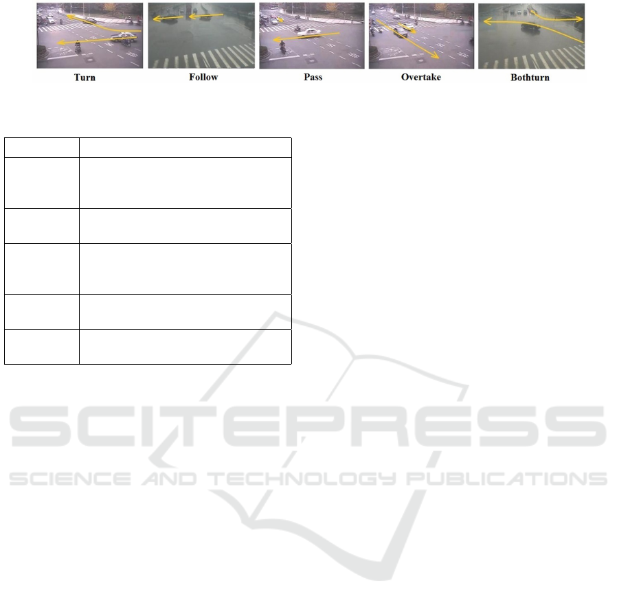
Figure 4: Sample of trafﬁc dataset (Lin et al., 2013).

Table 1: Deﬁnition of vehicles pair-activities.

Activity Description

Turn One vehicle moves straight and

another vehicle in another lane

turns right.

Follow One vehicle followed by another

vehicle on the same lane.

Pass One vehicle passes the crossroad

and another vehicle in the other di-

rection waits for green light.

Bothturn Two vehicles move in opposite di-

rections and turn right at same time.

Overtake A vehicle is overtaken by another

vehicle.

• We ﬁrst directly compare the performance of our

classiﬁcation method (described in Section 3.3)

against state-of-the-art quantitative and qualita-

tive methods (AlZoubi et al., 2017; Lin et al.,

2013; Lin et al., 2010; Ni et al., 2009; Zhou et al.,

2008) using the trafﬁc dataset presented in (Lin

et al., 2013).

• Then, we evaluate the performance of our super-

vised method on our dataset for vehicle-obstacle

interaction (AlZoubi and Nam, 2018) using com-

plete and predict trajectories.

All experiments were run on an Intel Core i7 desktop,

CPU@3.40GHz with 16.0GB RAM.

4.1 Experiment 1: Classiﬁcation of

Vehicle Activities

The state of the art pair-activity classiﬁcation met-

hods (AlZoubi et al., 2017; Lin et al., 2013) were

shown to outperform a number of other methods

(Zhou et al., 2008; Ni et al., 2009; Lin et al., 2010),

using the trafﬁc dataset presented in (Lin et al., 2013).

We therefore use these algorithms, trafﬁc dataset, and

ground truth, as a benchmark for evaluating our own

classiﬁcation method.

4.1.1 The Trafﬁc Dataset

The trafﬁc dataset was extracted from 20 surveillance

videos. Five different vehicles-activities, {Turn, Fol-

low, Pass, BothTurn, and Overtake} are represented

and corresponding annotations are provided. In total

there are 175 clips; 35 clips for each activity. The da-

taset includes x,y coordinates for the centroid of each

vehicle in each frame, a time-stamp t, and each clip

contains 20 frames. Figure 4 shows example frames

from the dataset, and Table 1 shows the deﬁnitions of

each activity in the dataset. To best of our knowledge

this is the only pair-wise trafﬁc surveillance dataset

publicly available.

4.1.2 Results for Vehicle Activity Classiﬁcation

We used the provided x,y coordinate pairs for each

vehicle as inputs, and constructed corresponding

QTC

trajectories for each video clip. Then, we

constructed corresponding image texture (I

) for each

QTC

trajectory using Algorithm 1. Figure 5 shows

images texture for ﬁve different interactions for the

samples in ﬁgure 4.

To determine the classiﬁcation rates using our

method, we used 5-fold cross validation. On each ite-

ration, we split the images texture (I) into training and

testing sets at ratio of 80% to 20%, for each class. The

training sets were used to parametrize our network

(Tra jNet). The test images texture were then clas-

siﬁed by our trained Tra jNet. Our results are shown

in Table 2, which includes comparative results obtai-

ned by (AlZoubi et al., 2017), (Lin et al., 2013), and

three other algorithms (Zhou et al., 2008; Ni et al.,

2009; Lin et al., 2010).The average error (AVG Error)

is calculated as the total number of incorrect classiﬁ-

cations (compared with the ground truth labeling) di-

vided by the total number of activity sequences in the

test set. Table 2 shows that our method outperforms

the other ﬁve, and is able to classify the dataset with

errors rate 1.16% and with a standard deviation 0.015.

4.2 Experiment 2: Classiﬁcation of

Vehicle-obstacle Interaction

We are primarily interested in the supervised recog-

nition of the relative interaction between the ego-

vehicle and its surroundings, which can help in the

decision making and predicting any potential collisi-

ons. We have constructed an extensive and expert-

Vehicle Activity Recognition using Mapped QTC Trajectories

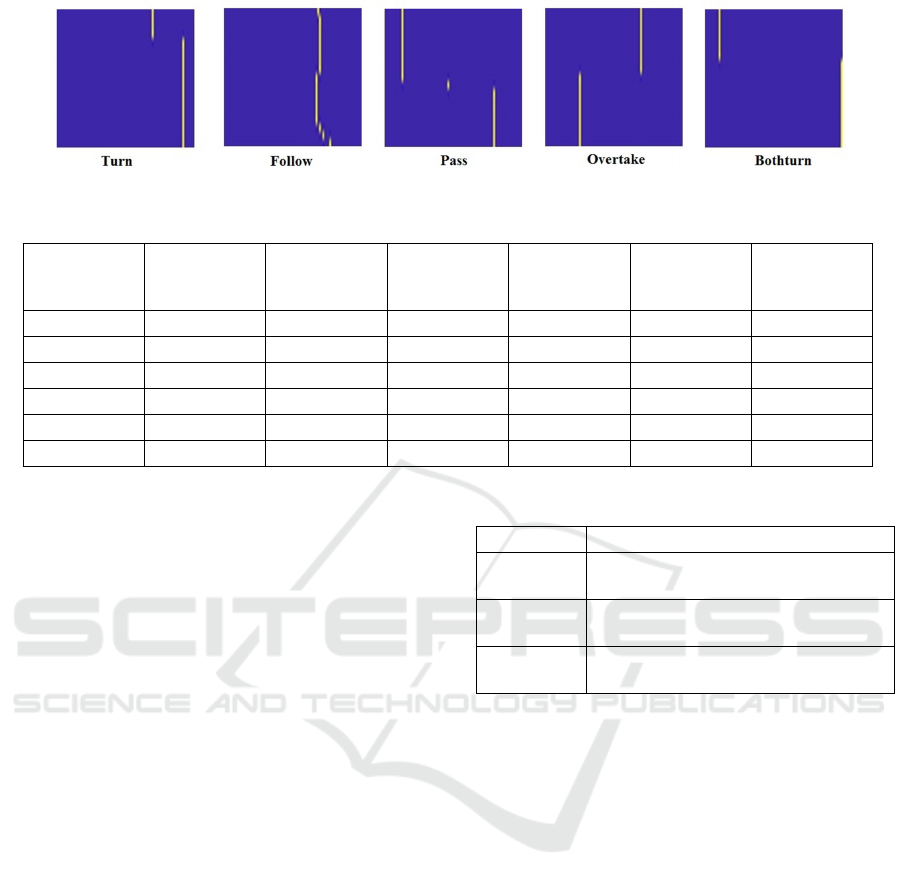
Figure 5: Images texture representation of trafﬁc dataset.

Table 2: Misclassiﬁcation error for different algorithms on the trafﬁc dataset.

Type Tra jNet NWSA (Al-

Zoubi et al.,

2017)

Heat-Map

(Lin et al.,

2013)

WF-SVM

(Zhou et al.,

2008)

LC-SVM (Ni

et al., 2009)

GRAD (Lin

et al., 2010)

Turn 2.9% 2.9% 2.9% 2.0% 16.9% 10.7%

Follow 0.0% 5.7% 11.4 % 22.9% 38.1% 15.4%

Pass 0.0% 0.0% 0.0% 11.7% 17.6% 15.5%

Bothturn 0.0% 2.9% 2.9% 1.2% 2.9% 4.2%

Overtake 2.9% 5.7% 5.7% 47.1% 61.7% 36.6%

AVG Error 1.16% 3.44% 4.58% 16.98% 27.24% 16.48

annotated dataset of vehicle-obstacle interactions,

collected in a simulation environment. This presents a

new challenging datasets, and therefore a new classiﬁ-

cation problem. In this section we evaluate the effecti-

veness and the accuracy of our supervised recognition

method and our driver model for trajectory prediction.

4.2.1 Setup

For our pair-wise vehicle-obstacle interactions and

our trajectory prediction model we collected data

through simulation. As we have focused on near col-

lision scenarios, there is not much available data, and

real testing would not be possible for the crash sce-

nario. Data was gathered using a simulation environ-

ment developed in Virtual Battlespace 3 (VBS3), with

the Logitech G29 Driving Force Racing Wheel and

pedals. Here a model of Dubai highway was used. We

consider a six lane road with an obstacle in the center

lane. The experiment consisted of 40 participants, all

of varying ages, genders and driving experiences. Par-

ticipants were asked to use their driving experience to

avoid the obstacle. A

Skoda Octavia was used in all

trails, and with maximum speed 50KPH. We recorded

the obstacle and ego-vehicle’s coordinates (the x, y

center position), velocity, heading angle, and distance

from each other. The generated trajectories were re-

corded at 10Hz.

4.2.2 Simulator Dataset

We have developed a new dataset for vehicle-

obstacle interaction recognition task (AlZoubi and

Table 3: Deﬁnition of vehicle-obstacle interactions.

Scenario Description

Left-Pass The ego-vehicle successfully passes

the object one the left.

Right-Pass The ego-vehicle successfully passes

the object one the right.

Crash The ego-vehicle and the obstacle col-

lide.

Nam, 2018). The dataset includes three subsets: the

ﬁrst (SS

) contains of 122 vehicle-obstacle trajecto-

ries of about 600 meters each (43,660 samples) for

training our trajectory prediction model. The second

subset (SS

) contains of 277 complete trajectories of

three different scenarios (67 crash, 106 left-pass, and

104 right-pass trajectories); which we consider to be

ground truth to evaluate the accuracy of our recog-

nition method and our trajectory prediction model.

Where the distance between the vehicle and the ob-

stacle (length of the trajectory) is 50 meters. Here

each scenario was observed and manually labelled by

two experts. Table 3 shows the deﬁnitions of each

scenario in the dataset. Figure 6 (a)-(c) shows sam-

ples of three different complete trajectories for Left-

Pass, Right-Pass and Crash, respectively. Finally, the

third subset (SS

) contains of 277 incomplete trajec-

tories. This subset is derived from the complete tra-

jectories (SS

) and used to evaluate our recognition

method and our trajectory prediction model. For tra-

jectory prediction we considered a distance of ε = 25

meters between the ego-vehicle and the obstacle. This

distance represented 50% of the complete trajectories.

Figure 6 (d) shows an example of the incomplete tra-

VISAPP 2019 - 14th International Conference on Computer Vision Theory and Applications

(a) Left-Pass (b) Right-Pass (c) Crash (d) Driver Model

Figure 6: Examples of scenarios from VBS3 with trajectory overlaid in red (a-c). The ego-vehicle is the green car and the

obstacle is the white car. (d) shows an example of the driver model, where the solid red line is the real trajectory and the

dashed line is the predicted trajectory.

0 10 20 30 40 50 60 70 80 90 100

101 Epochs

-2

-1

Mean Squared Error (mse)

Best Validation Performance is 0.014661 at epoch 95

Train

Validation

Test

Best

Figure 7: Training performance of driver model, and num-

ber of training iterations.

jectory for Right-Pass scenario, where the solid red

line is the real trajectory (25 meters) and the dashed

line is the predicted trajectory. Similarly, the third

subset contains 67 crash, 106 left-pass, and 104 right-

pass of incomplete trajectories with length 25 meters

each.

4.2.3 Evaluating Trajectory Prediction Model

We evaluated the accuracy of our driver model for

trajectory predictions. First, we train our FFNN

(Section 3.4) using SS1, containing 43,660 samples.

We split the samples in SS

into training, validation

and test subsets, 70%, 15% and 15%, respectively.

The training subset is used to calculate network weig-

hts, the validation subset to obtain unbiased network

parameters for training, and the test subset is used

to evaluate performance. Figure 7 shows the perfor-

mance of our network.

We evaluated the performance of our trajectory

prediction algorithm on SS

, consisting of 277 incom-

plete trajectories; we considered complete trajectories

(SS

) as the ground truth. Our test set contains 67

crash, 106 left-pass, and 104 right-pass trajectories.

Three examples from each scenario of the generated

trajectories are shown in ﬁgure 8. Here the trajec-

tory starts closest to the origin and travels diagonally,

from left to right. Human generated trajectories are

in green and red (where red is the ground truth), the

predicted trajectories are in blue. We calculate the tra-

jectory prediction error using the Modiﬁed Hausdorff

Distance (MHD) (Dubuisson and Jain, 1994). We se-

lected the MHD because its value increases monoto-

nically as the amount of difference between the two

sets of edge points increases, and it is robust to out-

lier points. Given the predicted trajectory T

and the

ground-truth trajectory as T

, we calculate our error

measure as:

M H D = min(d(T

),d(T

)). (7)

where d(∗) is the average minimum Euclidean distan-

ces between points of predicted and ground-truth tra-

jectories. The error across the entire test set is shown

in ﬁgure 9. Here the red line represents the mean error

and the bottom and top edges of the box indicate the

and 75

percentiles, respectively. The whiskers

extend to cover 99.3% of the data and the red plu-

ses represent outliers. Across all scenarios an average

error of 0.4m was observed, this amount of error is to-

lerable because the overall characteristic of the trajec-

tory is still captured, also, a typical highway lane can

be up to 3m, therefore variations can still be within

lane.

4.2.4 Results for Vehicle-obstacle Interaction

Classiﬁcation

We evaluated our recognition method on both com-

plete (SS

) and incomplete trajectories (SS

). First,

we used the x, y coordinate pairs for both the vehicle

Vehicle Activity Recognition using Mapped QTC Trajectories

120 125 130 135 140 145 150 155

x-axis (m)

185

190

195

200

205

210

215

220

225

230

y-axis(m)

Obstacle

Previous Trajectory

Predicted

Ground Truth

(a) Left-Pass–0.20m

130 135 140 145 150 155

x-axis (m)

185

190

195

200

205

210

215

220

225

y-axis(m)

Obstacle

Previous Trajectory

Predicted

Ground Truth

(b) Right-Pass–0.18m

50 55 60 65 70 75 80 85

x-axis (m)

100

105

110

115

120

y-axis(m)

Obstacle

Previous Trajectory

Predicted

Ground Truth

115 120 125 130 135 140 145 150 155

x-axis (m)

185

190

195

200

205

210

215

220

225

230

y-axis(m)

Obstacle

Previous Trajectory

Predicted

Ground Truth

(d) Left-Pass–0.69m

220 225 230 235 240 245 250 255

x-axis (m)

310

315

320

325

330

335

340

345

350

355

y-axis(m)

Obstacle

Previous Trajectory

Predicted

Ground Truth

(e) Right-Pass–0.14m

50 55 60 65 70 75 80 85

x-axis (m)

100

105

110

115

120

y-axis(m)

Obstacle

Previous Trajectory

Predicted

Ground Truth

(f) Crash–0.29m

Figure 8: Sample trajectories with associated errors, M H D. Two sets of example trajectories (top and bottom rows), covering

all three scenarios. (a)-(c) and (d)-(f) represent left-pass, right-pass, and, crash scenarios, respectively.

Left-Pass Right-Pass Crash

Scenario

0.5

1.5

2.5

Error from ground truth (m)

Figure 9: Errors (M H D) from scenarios, across SS3.

and the obstacle from SS

as inputs, and constructed

corresponding QTC

trajectories for each scenario.

Then, we constructed the corresponding image tex-

ture (I

) for each QTC

trajectory using Algorithm 1.

To determine the classiﬁcation rates using our method

on SS

dataset, we used 5-fold cross validation. On

each iteration, we split the images texture in SS

into

training and testing sets at ratio of 80% to 20% re-

spectively, for each class. The training sets were used

to parameterise our network (Tra jNet). The test data

was then classiﬁed by our trained Tra jNet. Our re-

sults are shown in Table 4, which includes results of

complete trajectories (Complete Traj). The average

error (AVG Error) is calculated as the total number

of incorrect classiﬁcations (compared with the ground

truth labeling) divided by the total number of activity

sequences in the test set.

Table 4: Misclassiﬁcation error for Complete and Predicted

Trajectories of Vehicle-Obstacle Interaction Dataset.

Type Complete

Traj (SS

)

Predicted

Traj (SS

)

Crash 0.0% 0.0%

Left-Pass 0.0% 0.0%

Right-Pass 0.0% 1.0%

AVG Error 0.0% 0.3%

For incomplete trajectories, we ﬁrst trained and

parametrized our FFNN (ﬁgure 3) using SS

. Then,

we used our driver model (Section 3.4) to predict the

complete trajectory for each scenario which resulted

in a new subset (SS

). Similarly, we used the x; y coor-

dinate pairs for both the vehicle and the obstacle from

as inputs, and constructed QTC

trajectories and

their corresponding images texture (I) for all scena-

rios. Figure 6 (d) shows a sample of predicted trajec-

tory. Again, to determine the classiﬁcation rates using

our method on SS

, we used 5-fold cross validation.

On each iteration, we split the images texture in SS

into training and testing sets at ratio of 80% to 20%,

for each class. The training sets were used to para-

meterise our network (Tra jNet). The test data was

then classiﬁed by our trained Tra jNet. Our results are

shown in Table 4, which includes results of predicted

trajectories (Predicted Traj). The results show that

our method has high classiﬁcation accuracy for both

complete and predicted trajectories. The total compu-

tation time of predicting and recognizing the scenario

that the vehicle is about to enter is 28 millisecond.

VISAPP 2019 - 14th International Conference on Computer Vision Theory and Applications

5 CONCLUSION AND

DISCUSSION

In this paper we have presented a new method for

predicting and classifying pair-activities of vehicles

using a new deep learning framework. Our method

uses the QTC representation, and we have constructed

corresponding image textures for each QTC trajec-

tory using one-hot vector. Our trajectory represen-

tation, successfully encodes different types of vehi-

cles activities, and is used as an input for Tra jNet.

Tra jNet offers a compact network for classifying

pair-wise vehicle interactions. We also demonstrate

how we efﬁciently used limited amount of dataset to

train Tra jNet, and achieved high accuracy classiﬁca-

tion rates across different and challenging datasets.

We have conducted direct comparisons against the

state-of-the-art qualitative (AlZoubi et al., 2017) and

quantitative (Lin et al., 2013) methods, which have

itself been shown to outperform other recent met-

hods. We have shown that our classiﬁcation met-

hod outperforms that developed by (Lin et al., 2013)

and (AlZoubi et al., 2017); for the classiﬁcation of

trafﬁc data, we achieved 1.16% error rate, compared

to 3.44%, 4.58%, 16.98%, 27.24%, and 16.48% of

(AlZoubi et al., 2017), (Lin et al., 2013), (Zhou et al.,

2008), (Ni et al., 2009) and (Lin et al., 2010), respecti-

vely.

We have also presented our vehicle-obstacle in-

teraction dataset for complete and incomplete scena-

rios, which provides a detailed and useful resource

for researchers studying vehicle-obstacle behaviors,

and is publicly available for download. We evaluated

our classiﬁcation method on this dataset, we achieved

0.0% and 0.3% for both complete and predicted sce-

narios datasets, respectively. This again demonstrates

the effectiveness of our activity recognition method.

To predict a full scenario from partial-observed one

we have presented a FFNN. We evaluated our trajec-

tory prediction method on the same vehicle-obstacle

dataset and we achieved average error of 0.4m.

Encouraged by our results, we plan to extend our

work by integrating our vehicles activity recognition

method with our ongoing project of autonomous vehi-

cle system to provide valuable information about the

type of the scenario the vehicle is in (or about to enter)

to increase the safety and to help in decision making

processes.

REFERENCES

Ahmed, S. A., Dogra, D. P., Kar, S., and Roy, P. P.

(2018). Trajectory-based surveillance analysis: A sur-

vey. IEEE Transactions on Circuits and Systems for

Video Technology.

AlZoubi, A., Al-Diri, B., Pike, T., Kleinhappel, T., and

Dickinson, P. (2017). Pair-activity analysis from video

using qualitative trajectory calculus. IEEE Transacti-

ons on Circuits and Systems for Video Technology.

AlZoubi, A. and Nam, D. (2018). Vehicle Ob-

stacle Interaction Dataset (VOIDataset).

https://ﬁgshare.com/articles/Vehicle Obstacle

Interaction Dataset VOIDataset /6270233.

Chavoshi, S. H., De Baets, B., Neutens, T., Delafontaine,

M., De Tr

e, G., and de Weghe, N. V. (2015). Mo-

vement pattern analysis based on sequence signatu-

res. ISPRS International Journal of Geo-Information,

4(3):1605–1626.

Deng, J., Dong, W., Socher, R., Li, L.-J., Li, K., and Fei-Fei,

L. (2009). Imagenet: A large-scale hierarchical image

database. In Computer Vision and Pattern Recogni-

tion, 2009. CVPR 2009. IEEE Conference on, pages

248–255. IEEE.

Dodge, S., Laube, P., and Weibel, R. (2012). Movement si-

milarity assessment using symbolic representation of

trajectories. International Journal of Geographical

Information Science, 26(9):1563–1588.

Dubuisson, M.-P. and Jain, A. K. (1994). A modiﬁed haus-

dorff distance for object matching. In Proceedings of

12th international conference on pattern recognition,

pages 566–568. IEEE.

Hanheide, M., Peters, A., and Bellotto, N. (2012). Analy-

sis of human-robot spatial behaviour applying a qua-

litative trajectory calculus. In RO-MAN, 2012 IEEE,

pages 689–694. IEEE.

Khosroshahi, A., Ohn-Bar, E., and Trivedi, M. M. (2016).

Surround vehicles trajectory analysis with recurrent

neural networks. In Intelligent Transportation Systems

(ITSC), 2016 IEEE 19th International Conference on,

pages 2267–2272. IEEE.

Krizhevsky, A., Sutskever, I., and Hinton, G. E. (2012).

Imagenet classiﬁcation with deep convolutional neu-

ral networks. In Advances in neural information pro-

cessing systems, pages 1097–1105.

Lin, W., Chu, H., Wu, J., Sheng, B., and Chen, Z. (2013). A

heat-map-based algorithm for recognizing group acti-

vities in videos. IEEE Transactions on Circuits and

Systems for Video Technology, 23(11):1980–1992.

Lin, W., Sun, M.-T., Poovendran, R., and Zhang, Z. (2010).

Group event detection with a varying number of group

members for video surveillance. IEEE Transacti-

ons on Circuits and Systems for Video Technology,

20(8):1057–1067.

Liu, W., Wang, Z., Liu, X., Zeng, N., Liu, Y., and Alsaadi,

F. E. (2017). A survey of deep neural network ar-

chitectures and their applications. Neurocomputing,

234:11–26.

Ni, B., Yan, S., and Kassim, A. (2009). Recognizing human

group activities with localized causalities. In Compu-

ter Vision and Pattern Recognition, 2009. CVPR 2009.

IEEE Conference on, pages 1470–1477. IEEE.

Ohn-Bar, E. and Trivedi, M. M. (2016). Looking at hu-

mans in the age of self-driving and highly automated

Vehicle Activity Recognition using Mapped QTC Trajectories

vehicles. IEEE Transactions on Intelligent Vehicles,

1(1):90–104.

Oquab, M., Bottou, L., Laptev, I., and Sivic, J. (2014). Le-

arning and transferring mid-level image representati-

ons using convolutional neural networks. In Computer

Vision and Pattern Recognition (CVPR), 2014 IEEE

Conference on, pages 1717–1724. IEEE.

Russakovsky, O., Deng, J., Su, H., Krause, J., Satheesh, S.,

Ma, S., Huang, Z., Karpathy, A., Khosla, A., Bern-

stein, M., et al. (2015). Imagenet large scale visual

recognition challenge. International Journal of Com-

puter Vision, 115(3):211–252.

Shi, Y., Tian, Y., Wang, Y., and Huang, T. (2017). Sequen-

tial deep trajectory descriptor for action recognition

with three-stream cnn. IEEE Transactions on Multi-

media, 19(7):1510–1520.

Shi, Y., Zeng, W., Huang, T., and Wang, Y. (2015). Lear-

ning deep trajectory descriptor for action recognition

in videos using deep neural networks. In Multime-

dia and Expo (ICME), 2015 IEEE International Con-

ference on, pages 1–6. IEEE.

Srivastava, N., Hinton, G., Krizhevsky, A., Sutskever, I.,

and Salakhutdinov, R. (2014). Dropout: a simple way

to prevent neural networks from overﬁtting. The Jour-

nal of Machine Learning Research, 15(1):1929–1958.

Szegedy, C., Liu, W., Jia, Y., Sermanet, P., Reed, S., Angue-

lov, D., Erhan, D., Vanhoucke, V., and Rabinovich, A.

(2015). Going deeper with convolutions. In Procee-

dings of the IEEE conference on computer vision and

pattern recognition, pages 1–9.

Van de Weghe, N. (2004). Representing and reasoning

about moving objects: A qualitative approach. PhD

thesis, Ghent University.

Xiong, X., Chen, L., and Liang, J. (2018). A new fra-

mework of vehicle collision prediction by combining

svm and hmm. IEEE Transactions on Intelligent

Transportation Systems, 19(3):699–710.

Xu, D., He, X., Zhao, H., Cui, J., Zha, H., Guillemard, F.,

Geronimi, S., and Aioun, F. (2017). Ego-centric traf-

ﬁc behavior understanding through multi-level vehi-

cle trajectory analysis. In Robotics and Automation

(ICRA), 2017 IEEE International Conference on, pa-

ges 211–218. IEEE.

Xu, H., Zhou, Y., Lin, W., and Zha, H. (2015). Unsuper-

vised trajectory clustering via adaptive multi-kernel-

based shrinkage. In Proceedings of the IEEE Interna-

tional Conference on Computer Vision, pages 4328–

4336.

Zhou, Y., Yan, S., and Huang, T. S. (2008). Pair-activity

classiﬁcation by bi-trajectories analysis. In Compu-

ter Vision and Pattern Recognition, 2008. CVPR 2008.

IEEE Conference on, pages 1–8. IEEE.

VISAPP 2019 - 14th International Conference on Computer Vision Theory and Applications