Visibility Estimation in Point Clouds with Variable Density

P. Biasutti

1,2,3

, A. Bugeau

, J-F. Aujol

and M. Br

edif

Univ. Bordeaux, LaBRI, INP, CNRS, UMR 5800, F-33400 Talence, France

Univ. Bordeaux, IMB, INP, CNRS, UMR 5251, F-33400 Talence, France

Univ. Paris-Est, LASTIG GEOVIS, IGN, ENSG, F-94160 Saint-Mand

e, France

Keywords:

3D Point Cloud, Visibility, Visualization, LiDAR, Dataset, Benchmark.

Abstract:

Estimating visibility in point clouds has many applications such as visualization, surface reconstruction and

scene analysis through fusion of LiDAR point clouds and images. However, most current works rely on

methods that require strong assumptions on the point cloud density, which are not valid for LiDAR point

clouds acquired from mobile mapping systems, leading to low quality of point visibility estimations. This

work presents a novel approach for the estimation of the visibility of a point cloud from a viewpoint. The

method is designed to be fully automatic and it makes no assumption on the point cloud density. The visibility

of each point is estimated by considering its screen-space neighborhood from the given viewpoint. Our results

show that our approach succeeds better in estimating the visibility on real-world data acquired using LiDAR

scanners. We evaluate our approach by comparing its results to a new manually annotated dataset, which we

make available online.

1 INTRODUCTION

Over the past decade, the use of 3D point clouds as

an alternative to meshes has been constantly growing.

A 3D point cloud simply consists in 3D positions, so-

metimes associated with supplementary information

such as its color, reﬂectance or normal. It can be con-

sidered as a sampling of continuous surface, provi-

ding a simpler representation than the full topology.

The estimation of the visibility of a point cloud

consists in assigning a label to each point of the scene:

visible if the point lies on an object that is directly vi-

sible from a given viewpoint, non-visible otherwise

(Fig. 1). This task is a typical step for various ap-

plications in computer graphics such as in surface re-

construction (Zach et al., 2007; Shalom et al., 2010;

Berger et al., 2017) in which estimating and remo-

ving points that are not visible from a given point of

view improves the interpolation and the approxima-

tion of the surface to recover. In point cloud rendering

and visualization (Pintus et al., 2011; Bouchiba et al.,

2017), the estimation of the visibility enables better

rendering performances as well as an improvement of

the scene understanding. For both application scena-

rios, the existing methods (Zach et al., 2007; Shalom

et al., 2010; Berger et al., 2017; Pintus et al., 2011;

Bouchiba et al., 2017) strongly rely on strict sampling

a. b. c. d.

Figure 1: Illustration of the visibility problem. (a) an optical

image corresponding to a view point, (b) the 3 main struc-

tures of the scene, (c) the projection of the acquired point

cloud seen from the same view point with same colors as in

(b), (d) the visibility errors brought by the projection (red

points should not be visible).

assumptions (Berger et al., 2017) (e.g. on point clouds

with constant density in terms of number of points per

cubic meters).

Recently, the development of acquisition systems

designed for acquiring urban scenes has been increa-

sing. In particular, Mobile Mapping Systems (MMS)

equipped with LiDAR (Light Detection And Ran-

ging) (Paparoditis et al., 2012; Geiger et al., 2013;

Maddern et al., 2017) have been widely used to sur-

vey cities, road, highways, etc. Those campaigns have

resulted in the production of large, unorganized point

clouds that provide precise 3D representations of the

urban environment. Due to the acquisition method,

these point clouds present high variation in their sam-

Biasutti, P., Bugeau, A., Aujol, J. and Brédif, M.

Visibility Estimation in Point Clouds with Variable Density.

DOI: 10.5220/0007308600270035

In Proceedings of the 14th International Joint Conference on Computer Vision, Imaging and Computer Graphics Theory and Applications (VISIGRAPP 2019), pages 27-35

ISBN: 978-989-758-354-4

pling and density. Most modern MMS also embed ad-

ditional materials, mostly optical images, which pro-

vide complementary information on the scene. The

multimodal aspect of these datasets may be levera-

ged to improve detection, classiﬁcation and prediction

techniques in urban environments (Benenson et al.,

2014; Eigen et al., 2014). Therefore, the fusion and

the registration of LiDAR and optical data became

critical as the use of multi-modal data deﬁnitely in-

creases performances of classiﬁcation/prediction al-

gorithms. Most of the recent related works strongly

rely on good visibility estimates (Mastin et al., 2009;

Guislain et al., 2017).

The majority of actual LiDAR/optical registra-

tion techniques that use visibility rely on estimation

techniques that were built for point clouds with strict

sampling assumptions that are not met by the LiDAR

data on which they operate. On the other hand, point

cloud rendering and surface reconstruction methods

presented above are not designed to perform on point

clouds with variable density. However, the quality of

the visibility estimation is a crucial preprocessing step

for multi-modal fusion applications as it drastically

lowers the ambiguities from one modality to another.

This work aims at studying a new method for esti-

mating the visibility in point clouds without constant

density acquired via MMS to improve the data fusion.

The paper contribution is threefold: ﬁrst, we pro-

pose a novel approach for the visibility estimation in

a point cloud that is robust to high density variati-

ons. This method is designed to be fully automatic

and to perform well on any types of 3D point clouds.

The second contribution of this article is a new visi-

bility dataset of over 1 million annotated points for

testing the performances of visibility estimation met-

hods. This dataset, as well as the code for our method,

are made publicly available online. The third contri-

bution of this dataset is a full numerical and visual

comparison between our method and other state-of-

the-art methods.

The paper is organized as follows: ﬁrst, a brief

overview of the related work is presented. Then, the

methodology of the method is explained. Finally,

evaluation and results are shown and a conclusion is

drawn.

2 RELATED WORKS

There has been many contributions to the state-of-the-

art techniques for the estimation of the visibility of a

point cloud given a certain viewpoint. In this section,

we brieﬂy overview the methods that are most rele-

vant to our work.

Surface Reconstruction based. One intuitive way

to compute the visibility of a point cloud is to recon-

struct the surface. Indeed, the projection of the sur-

face as a depth map may be used to estimate which

points are not visible. Some methods do not require

prior knowledge of the visibility and can therefore be

used for visibility estimation. Surface smoothness ap-

proaches (Lipman et al., 2007; Xiong et al., 2014)

approximate the surface by locally deﬁning operators

that weigh surrounding points in order to estimate the

local surface. This constrains the reconstructed sur-

face to ﬁt the point cloud as close as possible while

ensuring a certain level of smoothness and preser-

ving sharp features. To deal with large amounts of

missing data, Volume smoothness techniques (Tagli-

asacchi et al., 2011; Huang et al., 2013) exploit the

prior of smooth variation of the volume of the recon-

structed surface. Unfortunately, these methods are ba-

sed on strong prior of uniform sampling of the point

cloud, which is not suitable for MMS LiDAR point

clouds. Primitive based methods (Schnabel et al.,

2009; Lafarge and Alliez, 2013) aim at ﬁtting geome-

tric shapes (i.e. planes, spheres, cylinders, boxes, etc.)

in order to reconstruct the scene. However, the com-

plex shapes that can be met in real world scene often

jeopardize the results of such methods. Finally, Glo-

bal regularity approaches (Li et al., 2011a; Li et al.,

2011b; Monszpart et al., 2015) take advantage of the

repeatability of certain parts of the scene. These met-

hods have shown great strength for the reconstruction

of individual regular shapes such as facades or roads

but underperform on realistic complete scenes. Alt-

hough each technique provides satisfying results on

speciﬁc scenarios, surface reconstruction is a difﬁcult

problem, which often requires additional information,

such as normals, sufﬁciently dense input and uniform

sampling.

Convex Hull based. Some methods estimate the vi-

sibility based on the local geometry of the 3D point

cloud. Based on the raw point cloud (i.e. only 3D

positions), (Katz et al., 2007) proposes an approach

for estimating which part of the point cloud is not

self-occluded given a certain viewpoint. This method

admits to perform better on closed shapes. A spher-

ical inversion is performed on the point cloud. The

convex hull of the inverted point cloud augmented by

the viewpoint position is computed. Then, points that

are lying on the convex hull are considered visible,

and the rest of the point cloud as non-visible. The

acceptance of concave features is tuned by the sphere

radius, which is a global parameter so that this met-

hod strongly relies on a uniform sampling of the point

cloud. Later, this method was improved to handle

VISAPP 2019 - 14th International Conference on Computer Vision Theory and Applications

small changes in the sampling corresponding to noisy

acquisitions (Mehra et al., 2010), but still relies on

constant density in the point cloud. Moreover, the

computational cost of the convex hull (Barber et al.,

1996) can rapidly increase depending on the wanted

concavity. Finally, (Katz et al., 2007; Mehra et al.,

2010) are both designed to perform on point clouds

that represent closed shapes, acquired from all directi-

ons, which is not realistic in urban scenarios where

MMS are not able to scan all surfaces.

Likelihood based. Different methods aim at esti-

mating the likelihood of a point to be visible given

a point of view, by considering its neighborhood. The

most common methods rely on the estimation of visi-

bility cones in screen-space (Shalom et al., 2010), and

more recently (Pintus et al., 2011). For each point,

a visibility cone is estimated, where the apex of the

cone is the given viewpoint. The aspect of the cone

is directly related to the visibility. Thus, a point that

belongs to a wide cone is more likely to be visible

than a point that belongs to a narrow cone. However,

the threshold on how open a cone should be in order

to consider the point visible strongly depends on the

point cloud, and can be hard to set.

In this paper, we propose an automatic screen-

space method for estimating the visibility of points in

a point cloud given a viewpoint. This method makes

no assumptions on the sampling or the density of the

point cloud and can therefore performed on any point

cloud.

3 VISIBILITY ESTIMATION

METHOD

The ﬁrst contribution of this paper is a method for

estimating visibility in a 3D point cloud that is robust

to high sampling variations.

As illustrated in Fig. 2, points from two objects lo-

cated at different distances from the given viewpoint

overlap in the image plane once projected. In this con-

text, a point is visible only if it lies on the closest ob-

ject and occluded otherwise. From this observation,

we propose an algorithm that considers the neighbor-

hood of a point in screen-space in order to estimate

whether this point lies on the closest object or not.

The algorithm consists in 4-steps detailed hereafter.

Projection to Screen-space. Let P be a 3D point

cloud, and Φ a viewpoint such that any 3D point

Figure 2: Illustration of notations in 3D and in the screen-

space. Blue points corresponds to the points lying on the

closest object while red points lies on the farthest object.

Although the blue points and red points are well separated

in 3D, they overlap in screen-space.

(a) (b)

Figure 3: Illustration of the depth and of the closest points.

(a) d

corresponds to the depth between P and the center of

the viewpoint, (b) shows an example of the N closest points

in screen-space (N = 6).

P =









∈ P can be projected as a point p =





∈

in the image plane of the viewpoint Φ. The rela-

tion between P and p is illustrated on Fig. 2. We also

deﬁne d

as the depth of the point p. It corresponds to

the 3D Euclidean distance between P and the center

of the viewpoint as illustrated Fig. 2(a).

Neighbors Computation. We deﬁne N (p) as the

set of the N nearest neighbor points of p in the image

plane as explained in Fig. 3(b) The N (p) set can be

computed using any K-NN alogrithm with a Eucli-

dean distance. The use of the K-NN algorithm de-

ﬁned in (Friedman et al., 1977) ensures logarithmic

computation time while being parallelizable.

Visibility Estimation. For each point, we want to

determine if it lies on the object in its neighborhood

that is the closest to the viewpoint. If so, we can con-

sider it as visible. To that end, we compare its posi-

tion to the closest and the farthest point of its neig-

hborhood. We deﬁne the visibility of each point as

follows:

= e

−

(

−d

min

)

(

max

−d

min

)

(1)

where

min

= min

q∈N (p)

, d

max

= max

q∈N (p)

Visibility Estimation in Point Clouds with Variable Density

The visibility estimation of each point p ∈ P

now given by α

∈ [0, 1], where α

= 0 means that p

is occluded and α

= 1 means that p is surely visible.

Binarization. The visibility of a point cloud being a

binary notion, we propose the following binarization

of α



1 if α

≥

0 otherwise.

(2)

with

α =

Card(P

)

∑

p∈P

the mean of the estimated vi-

sibilities. Note that various

α values have been tested

such as

α = 0.5 or the median value of the estimated

visibilities as discussed Section 5. However, in our

experiments on LiDAR data, the mean value remains

the best threshold. When point clouds have constant

densities,

α = 0.99 appears to be more adequate.

4 VISIBILITY ESTIMATION

DATASET FOR LiDAR POINT

CLOUDS

The evaluation of visibility estimation techniques has

mostly been done either by visual analysis or by com-

parison to degradated synthetic models. In (Shalom

et al., 2010; Katz et al., 2007), visual results are dis-

played to show the qualitative performances of each

algorithm. In (Mehra et al., 2010), small degradati-

ons on synthetic model are applied in order to build

groundtruths. Although these methods of evaluation

provide convincing results, they do not provide com-

plete and objective quantitative measures on real data.

Real data, such as LiDAR, differ from synthetic data

in two aspects. The ﬁrst difference is that the point

cloud density is highly variable on real data depen-

ding on the distance to the sensor, while constant on

synthetic data. The second one is that real urban data

only acquire partial representations of each object of

the scene as the sensor does not see objects from every

possible viewpoints. On the other hand, the synthe-

tic data presented in the related works (Shalom et al.,

2010; Katz et al., 2007; Mehra et al., 2010) are al-

ways complete 3D objects, which can be seen from

any viewpoint. To our knowledge, we give here the

ﬁrst annoted dataset on real urban LiDAR data, which

makes the second contribution of this paper.

4.1 Overview of the Dataset

We propose a manually annotated dataset containing

over a 1 million points with the label 1 or 0 depen-

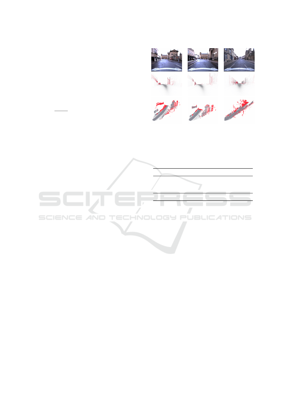
Figure 4: Overview of the proposed dataset. First row: op-

tical image corresponding to each viewpoint. Second row:

point cloud once projected in the image domain, where red

pixels correspond to occluded points. Third row: 3D visua-

lization of each point cloud, with the same color code than

in the second row.

Table 1: Content of the visiblity estimation dataset.

Points Visibility Farthest point Size

Scene #1 337384 55.5% 75.8m 20.6Mb

Scene #2 247682 57.0% 54.3m 15.1Mb

Scene #3 463531 65.9% 179.2m 28.3Mb

Total 1048597 59.46% - 64Mb

ding on if the points are visible or not. This data-

set has been obtained by manually labeling 3 point

clouds acquired by the RobotCar system (Maddern

et al., 2017) at different locations, in urban environ-

ment. Two of these point clouds are acquired several

meters from one another in order to test the stability of

visibility estimation methods. The third point cloud

corresponds to another location and covers a much

wider area which enables testing the limit of methods

in case of large distances (> 100m).

Annotations were done manually by comparing

the projections of the point clouds to the optical ima-

ges acquired at the same viewpoints. Fig. 4 presents

an overview of the produced dataset. The ﬁrst row il-

lustrates each scene as acquired from the optical sen-

sor at each viewpoint. The second row shows the pro-

jections of each point cloud in the image domain (with

the calibration matrices provided by the Robotcar da-

taset (Maddern et al., 2017)), where occluded points

are highlighted in red. Finally, the third row shows a

3D visualization of each point cloud, with same color

code than above. It illustrates the amount of points

to be processed as well as the size of the scenes. The

statistics of the dataset are summed up in Table 1. The

dataset proposes different levels of visible / occluded

points, as well as different size of the scene.

VISAPP 2019 - 14th International Conference on Computer Vision Theory and Applications

This dataset is publicly available online

. The ar-

chive contains 3 text ﬁles in the .xyz format that cor-

respond to each point cloud. In each ﬁle, a line cor-

responds to [x, y, z, u, v, label] where x, y, z are the 3D

coordinates of the point, u, v are the 2D coordinates of

the point when projected into φ and label is the visibi-

lity label (0 for occluded points, 1 for visible points).

To ensure good understanding of each of the 3 sce-

nes, we also provide the optical RGB image of size

1280 × 960px associated to each viewpoint.

5 EXPERIMENTS & RESULTS

In order to evaluate the performances of our visibility

estimation method, we ﬁrst perform a full numerical

and visual comparison between our method and other

state-of-the-art methods on (1) the proposed visibility

dataset, (2) a point cloud with constant density. Next,

we show application of our method to data fusion by

performing point cloud colorization from RGB ima-

ges. All the algorithms are run on Matlab 2018a with

a 3.5Ghz CPU.

5.1 Evaluation on the Visibility

Estimation Dataset

Using our new annotated dataset, we propose an eva-

luation with two state-of-the art methods, and with

our proposed model, against a groundtruth. For each

(a) Point cloud (b) Ground truth

Figure 5: Results of visibility estimation on the ﬁrst scene of

our visibility estimation dataset.. (a) the point cloud where

the heat of the color is proportional to the depth, (b) is the

annotated point cloud (red: visible, grey: non-visible), (c)

HPR result and (d) our result. The result brought by HPR

estimates too many visible points, whereas our method pro-

vides a result that is very close to the groundtruth.

http://www.labri.fr/perso/pbiasutt/Visibility/

method, we set all the parameters to its optimal va-

lue (e.g. the parameters that gives best results against

the groundtruth). In our case, we set N = 75 and we

detail results for different

α values. We measure the

efﬁciency of each method by computing the following

metric:

S(P ) =

Card(P )

∑

P∈P

× GT

(3)

where GT

corresponds to the annotation of the point

P (0 or 1, occluded or visible respectively). This me-

tric aims at capturing the percentage of correctly la-

beled points provided by each method. The results of

this evaluation are displayed in Table 2.

Table 2 demonstrates that our algorithm outper-

forms each compared methods for the 3 scenes. The

best scores are obtained by setting the threshold

equal to the mean of visibility estimations for our met-

hod. This observation is explanable. Indeed, as men-

tionned above, LiDAR aquisitions only capture pieces

of the scene. Thus, objects are represented by one of

their face only which makes them well separated from

one another. In this sense, when an object overlaps an

other in screen-space, the mean of the visibility esti-

mations usually represents the visibility of a point that

would be in between those two objects. If a point has

a visibility estimation above this threshold, it is likely

to fall on the closest object, otherwise, it is occluded.

Therefore, the mean value can be used when working

on LiDAR point clouds because of the way objects are

separated from one another, making the method fully

automatic in this context.

We also demonstrate that our method operates fas-

ter than any other tested method with the ability of

treating the whole dataset in less than a second. Mo-

reover, the code is run on a single CPU. Among the 4

steps of the algorithm, the computation of the K-NN

is the most time consuming (about 86% of the total

running time). Therefore, one can expect much fas-

ter running times by operating on GPU with parallel

implementation of the K-NN algorithm.

The problem of visibility estimation is a classiﬁ-

cation problem with two classes: visible and occluded

points. Therefore, we enrich our evaluation by com-

puting typical classiﬁcation metrics for each method

and display them in Table 3. For each metric, the best

scores are obtained using our method. In particular,

our method with

α = 0.5 maximizes the true-positives

and minimizes the false-negatives. On the opposite,

our method with

α as the median of the estimati-

ons maximizes the false-positives and true-positives.

Once again, using our method with

α as the mean

of the estimations provides a good tradeoff between

true-positives/true-negatives and false-positives/false-

negatives. On the other hand, (Katz et al., 2007) and

Visibility Estimation in Point Clouds with Variable Density

Table 2: Comparison of the scores of two state-of-the art and our visibility estimation methods on our visibility estimation

dataset.

HPR (Katz et al., 2007) Cone (Pintus et al., 2011) Ours Ours Ours

Threshold optimal optimal

α = 0.5 α

median α

mean

POV #1 74.09% 68.76% 90.15% 86.35% 90.96%

POV #2 69.09% 61.68% 86.95% 86.78% 88.39%

POV #3 81.55% 75.58% 82.21% 76.35% 83.75%

Average 74.91% 68.67% 86.43% 83.16% 87.70%

Total time 7.82s 1.53s 0.91s 1.03s 0.91s

Table 3: Comparison of the different methods for point cloud visibility classiﬁcation.

HPR (Katz et al., 2007) Cone (Pintus et al., 2011) Ours Ours Ours

Threshold optimal optimal

α = 0.5 α

median α

mean

True-positive 89.54% 85.16% 95.45% 78.31% 88.23%

False-positive 18.84% 17.78% 10.78% 3.66% 5.15%

False-negative 6.26% 8.61% 2.79% 13.18% 7.14%

True-negative 54.47% 56.24% 72.45% 90.80% 86.93%

Accuracy 85.16% 84.27% 92.52% 90.94% 93.44%

F1-score 87.71% 86.59% 93.37% 90.29% 93.49%

(Pintus et al., 2011) tend to over-estimate the visibility

of each point, resulting in many occluded points being

label as visible. This is expressed by the very high

percentage of false-positive. We computed accuracy

and the F1-score of each method against the ground

truth. For both, our method with

α as the mean of the

estimation achieves, once again, the best results.

For the task of data-fusion, it is often preferable to

discard the maximum of occluded points (Bevilacqua

et al., 2017). Therefore, the number of false-positives

has to be kept as low as possible. In this sense, our

method provides very satisfactory results, especially

using the

α as the mean of estimations when working

on LiDAR data.

We conclude this evaluation on LiDAR data by a

visual analysis of the results of the different methods.

Fig. 5 shows the results of the visibility estimations

visualized in 3D. For each result, the dark cone in the

bottom left corner represents the viewpoint. Fig. 5(a)

shows the point cloud colorized with the depth toward

the viewpoint (cold colors for close points, hot co-

lors for far points). Fig. 5(b) shows the annotated

groundtruth for this scene, where red points are points

that are visible from the viewpoint and dark points

are supposed to be occluded. Fig. 5(c) and 5(d) are

the results of HPR (Katz et al., 2007) and our method

(with

α set as the mean of estimations) respectively.

We can see that HPR (Katz et al., 2007) estimates too

many points as visible points, especially on the clo-

sest points. On the opposite, our method succeeds in

discarding occluded points, and provides a result that

is very close to the groundruth.

We also illustrate these results as seen from the as-

(a) Optical image (b) Groundtruth

Figure 6: Results of the visibility estimations on the ﬁrst

scene of the dataset in screen-space. (a) the optical image

associated with the point of view, (b) visible points with

respect to our annotation, (c) HPR result and (d) ours. Red

points in (c) and (d) correspond to misestimated points.

sociated viewpoint in Fig. 6. For better understanding

purpose, Fig. 6(a) shows an image acquired from the

same viewpoint. In Fig. 6(b), we only display visible

points of the groundtruth. Fig. 6(c) and 6(d) shows

the results of HPR (Katz et al., 2007) and our met-

hod respectively. We can see once again that HPR

(Katz et al., 2007) labels too many occluded points as

visible and fails to distinguish foreground from back-

ground objects. This is mostly due to the fact that this

scene presents very high variations of density. In par-

ticular, the center of the road concentrates a very high

density of points as the sensor is close from the road.

Therefore, the convex-hull has to be relaxed enough

to ﬁt this region of the point cloud, which leads to vi-

VISAPP 2019 - 14th International Conference on Computer Vision Theory and Applications

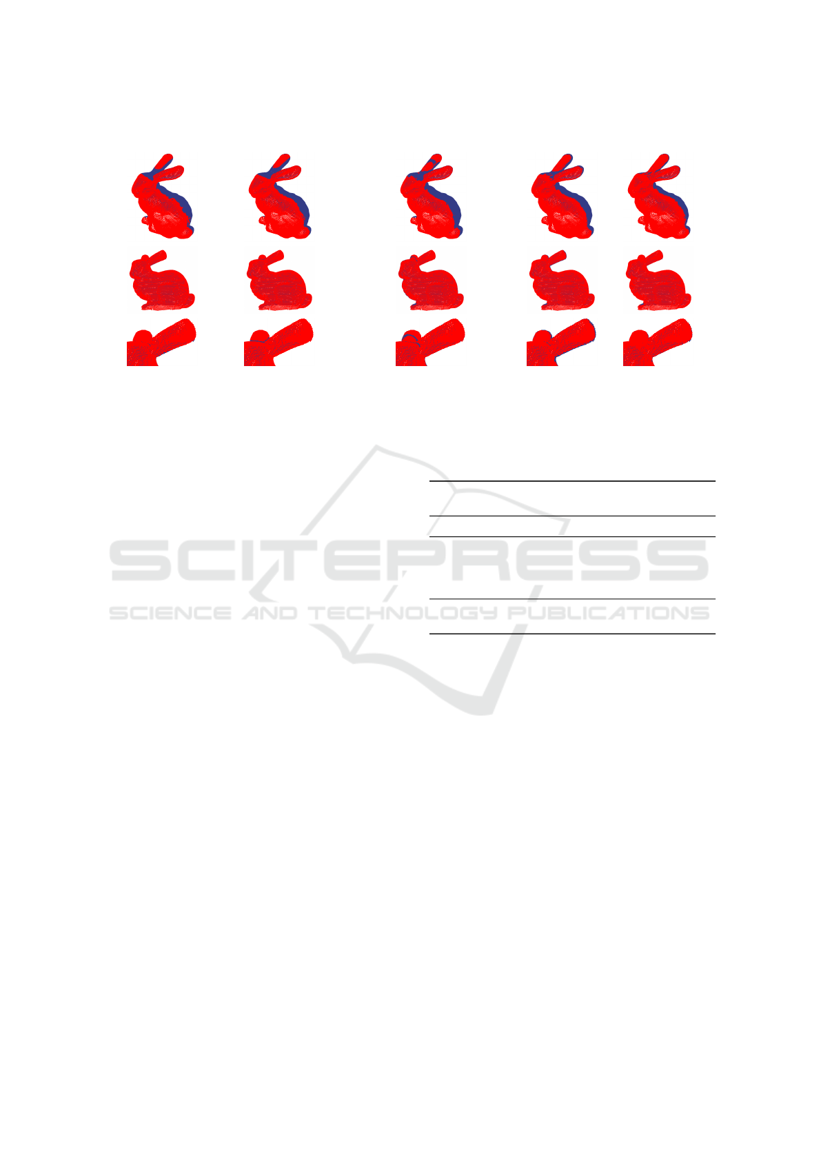
Ground truth HPR (Katz et al., 2007) Cone (Pintus et al., 2011) Ours (

α = 0.99) Ours (mean)

Figure 7: Visual comparison of the visibility estimation from different methods on a point cloud with constant and high

density. Each column corresponds to one method. Rows are respectively: the results in 3D, the results in 2D (seen from

the viewpoint), and a zoom of the 2D result focused on the ear region. The 3 methods succeed very well in estimating the

visibility. Our methods lacks of precision for points that are tangent to the viewpoint as can be seen on the last row.

sual abberations on regions with lower density. Our

method succeeds better results this scene, which de-

monstrates its robustness against high density variati-

ons.

5.2 Evaluation on Constant Density

Point Cloud

In previous section, we demonstrated that our method

performs better than other methods for point clouds

with high density variations. In this section, we aim

at showing that our method remains competitive on

constant density point clouds. The Stanford Bunny

model is a point cloud (from the Stanford University

CG Laboratory) that was created by merging 10 depth

aquisitions of a real object and equalizing the den-

sity of the fused point cloud. The ﬁnal point cloud is

composed of 31655 points. As each depth acquisition

only acquires points that are visible from a single vie-

wpoint, we created a groundtruth by comparing the

ﬁnal point cloud to the points that were aquired at a

certain viewpoint. Criterion (3) and classiﬁcation me-

trics have been computed for our method and state-of-

the-art methods. Results are displayed in Table 4.

Here, the point cloud is of constant density and

represents a very smooth object as illustrated Fig. 7.

This is a scenario that is perfectly adequate for the

HPR algorithm, which shortly outperforms the two

other methods. Our method underperforms only by

about 1 percent but still remains very efﬁcient on

these types of data. Compared to the two other met-

hods, our method fails on tangential points that are

located at the boundaries of the projection of the ob-

ject as it is presented on the last row of Fig. 7. This

Table 4: Comparison of the scores of the different methods

on constant density point cloud.

HPR Cone Ours Ours

Threshold optimal optimal

α = 0.99 α

mean

Score (Eq. (3)) 96.57% 93.75% 95.23% 93.02%

True-positive 95.17% 88.63% 94.44% 98.07%

False-positive 1.15% 0.88% 2.14% 6.07%

False-negative 2.28% 5.37% 2.63% 0.91%

True-negative 97.82% 98.33% 95.95% 88.50%

Accuracy 98.25% 96.76% 97.56% 96.40%

F1-score 98.23% 96.59% 97.54% 96.57%

is mostly due to the fact that on tangential points, the

neighborhood covers only a small area, thus the diffe-

rence between foreground and background is hard to

set. These artifacts are limited when using the mean

of estimation as visibility threshold, but it increases

false-positives. Table 4 also illustrates the classiﬁca-

tion metrics. We can see that all tested methods re-

ach very good levels of accuracy and F1-score. Our

method succeeds better when

α = 0.99 than when

using the mean value. Indeed, for complete object,

there is no separation between foreground object and

background object as was the case for LiDAR point

clouds. Thus, only points with high likelihood should

be kept to improve results, which justiﬁes

α = 0.99.

Finally, Table 4 assesses that all methods limit the

appearance of false-positives while ensuring to gather

as many visible points as possible. To that end, HPR

and our method succeed the best true-positive/false-

positive ratio, which is ideal for data-fusion purposes,

as discussed in next section.

Visibility Estimation in Point Clouds with Variable Density

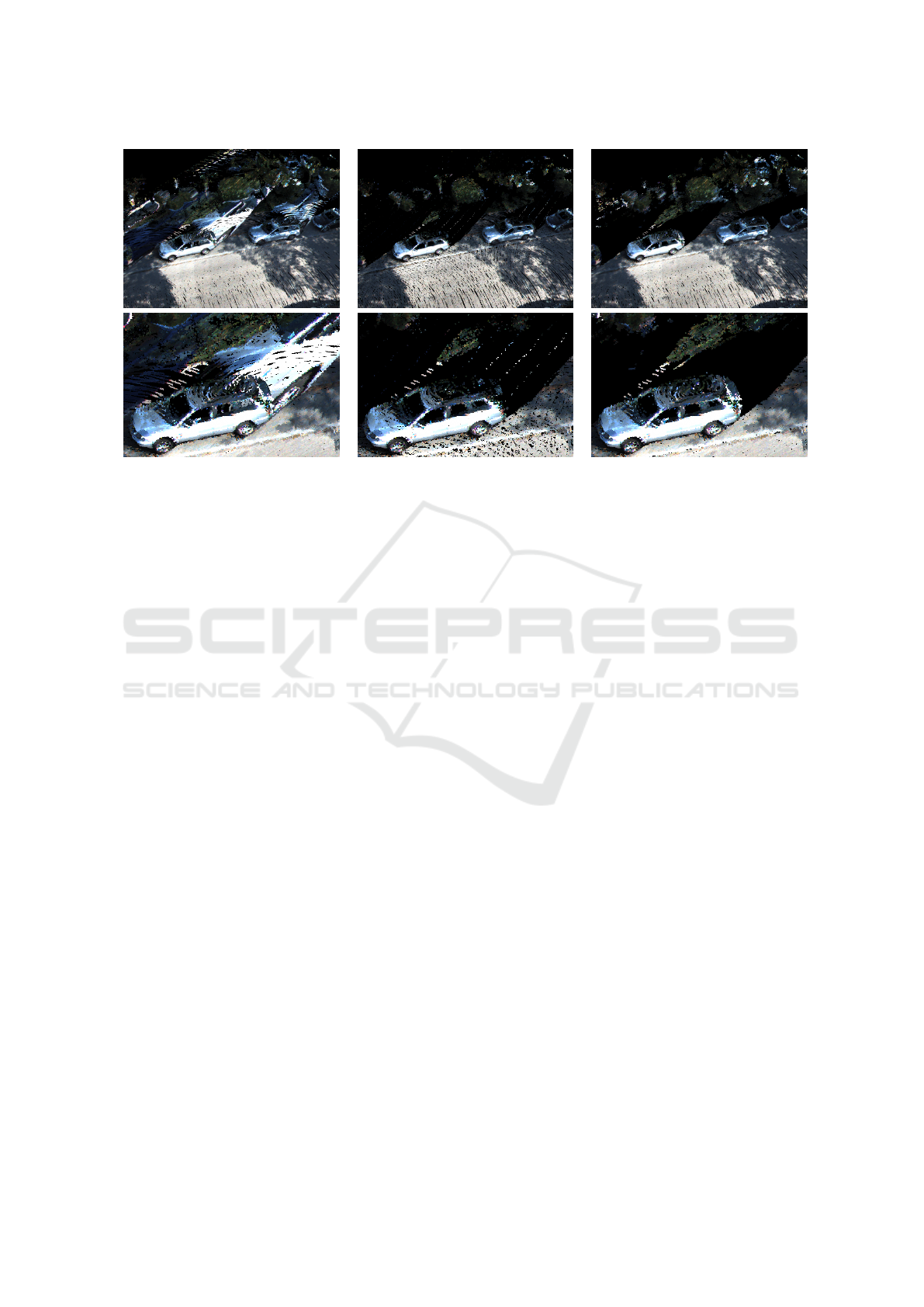
(a) (b) (c)

Figure 8: Comparison of the colorization of point clouds using RGB images. (a) colorization without any visibility informa-

tion, (b) colorization with HPR (Katz et al., 2007) for the visibility estimation, (c) colorization with our visibility estimation

method. The result provided by our method presents no artifacts on occluded areas, especially behind cars compared to the

two other results.

5.3 Example of Application to Data

Fusion

To conclude our experiments, we show the interest

of our visibility estimation for the task of data fu-

sion. Using the KITTI dataset (Geiger et al., 2013),

we aim at colorizing a 3D LiDAR point cloud acqui-

red in a street using only RGB images. Each point

is projected in the image domain of the closest image

(e.g. the image that was acquired at the closest posi-

tion from the point). The point then takes the color of

the pixel it projects into only if it is considered visible.

Fig. 8 presents the result of the colorization on a point

cloud composed of 3289533 points, and is colorized

using 40 RGB images. Fig. 8(a) shows the coloriza-

tion result where all points are considered visible. We

can see that artifacts appear as the colors do not match

the objects. This is particularly noticeable behind cars

where the ground points take the color of the car. Fig.

8(b) displays the colorization result where the visibi-

lity is estimated using HPR (Katz et al., 2007). There,

some artifacts appear behind cars as the convex-hull

go through the glasses of the car. Moreover, this met-

hod discards many visible points on the ground and

behind cars compared to our method (about 17% less

points are colorized). Fig. 8(c) presents the coloriza-

tion result using our visibility estimation method. We

can see that the artifacts behind cars have completely

disappeared, while keeping most of the visible points.

Finally, due to the number of points, the visibility es-

timation using HPR (Katz et al., 2007) for each vie-

wpoint takes an average of 10.9 seconds whereas our

method processes the point cloud at each viewpoint in

about 1.2 seconds.

6 CONCLUSION &

PERSPECTIVES

In this paper, we have proposed a novel method for

the visibility estimation in a point cloud. Compared

to other methods from literature, this method is very

robust to high variations of density. By considering

the closest neighbors of each point in screen-space,

we deﬁned a criterion in order to automatically deter-

mine the visibility of each point. We have also propo-

sed a new annotated dataset for testing the efﬁciency

of point cloud visibility algorithms on real LiDAR ur-

ban data. This dataset is composed of over a million

manually annotated points. Finally we have compa-

red our method to state-of-the-art methods. We have

validated that our method signiﬁcantly outperforms

existing methods on real urban data. Although our

method was speciﬁcally designed for the estimation

of visibility on point cloud with various density (such

as LiDAR point clouds), we have also demonstrated

that it still remains competitive on point clouds with

constant density.

In the future, we would like to focus on the eva-

luation of our method against photogrammetric point

clouds, for tasks such as view generation. We also

VISAPP 2019 - 14th International Conference on Computer Vision Theory and Applications

would like to improve LiDAR / Optic fusion thanks

to the visibility estimation.

ACKNOWLEDGEMENT

This study has been carried out with ﬁnancial sup-

port from the French State, managed by the French

National Research Agency (ANR GOTMI) (ANR-16-

CE33-0010-01). This project has also received fun-

ding from the European Union’s Horizon 2020 re-

search and innovation programme under the Marie

Skłodowska-Curie grant agreement No 777826.

REFERENCES

Barber, C. B., Dobkin, D. P., and Huhdanpaa, H. (1996).

The quickhull algorithm for convex hulls. ACM Tran-

sactions on Mathematical Software, 22(4):469–483.

Benenson, R., Omran, M., Hosang, J., and Schiele, B.

(2014). Ten years of pedestrian detection, what have

we learned? In ECCV European Conference on Com-

puter Vision, pages 613–627.

Berger, M., Tagliasacchi, A., Seversky, L. M., Alliez, P.,

Guennebaud, G., Levine, J. A., Sharf, A., and Silva,

C. T. (2017). A survey of surface reconstruction from

point clouds. In Computer Graphics Forum, pages

301–329.

Bevilacqua, M., Aujol, J.-F., Biasutti, P., Br

edif, M., and

Bugeau, A. (2017). Joint inpainting of depth and re-

ﬂectance with visibility estimation. ISPRS Journal of

the Photogrammetry, Remote Sensing and Spatial In-

formation Sciences, 125(1):16–32.

Bouchiba, H., Groscot, R., Deschaud, J.-E., and Goulette,

F. (2017). High quality and efﬁcient direct rendering

of massive real-world point clouds. In Eurographics

Annual Conference of the European Association for

Computer Graphics, pages 1–6.

Eigen, D., Puhrsch, C., and Fergus, R. (2014). Depth map

prediction from a single image using a multi-scale

deep network. In Advances in neural information pro-

cessing systems, pages 2366–2374.

Friedman, J. H., Bentley, J. L., and Finkel, R. A. (1977).

An algorithm for ﬁnding best matches in logarithmic

expected time. ACM Transactions on Mathematical

Software, 3(3):209–226.

Geiger, A., Lenz, P., Stiller, C., and Urtasun, R. (2013). Vi-

sion meets robotics: The KITTI dataset. IJRR Inter-

national Journal of Robotics Research, 32(11):1231–

1237.

Guislain, M., Digne, J., Chaine, R., and Monnier, G. (2017).

Fine scale image registration in large-scale urban LI-

DAR point sets. CVIU Computer Vision and Image

Understanding, 157(12):90–102.

Huang, H., Wu, S., Cohen-Or, D., Gong, M., Zhang, H.,

Li, G., and Chen, B. (2013). L1-medial skeleton of

point cloud. In ACM Transactions on Graphics, pages

65–72.

Katz, S., Tal, A., and Basri, R. (2007). Direct visibility of

point sets. In ACM Transactions on Graphics, pages

24–36.

Lafarge, F. and Alliez, P. (2013). Surface reconstruction

through point set structuring. In Computer Graphics

Forum, pages 225–234.

Li, Y., Wu, X., Chrysathou, Y., Sharf, A., Cohen-Or, D.,

and Mitra, N. J. (2011a). Globﬁt: Consistently ﬁtting

primitives by discovering global relations. In ACM

Transactions on Graphics, pages 52–64.

Li, Y., Zheng, Q., Sharf, A., Cohen-Or, D., Chen, B., and

Mitra, N. J. (2011b). 2D-3D fusion for layer decom-

position of urban facades. In ICCV IEEE Internatio-

nal Conference on Computer Vision, pages 882–889.

Lipman, Y., Cohen-Or, D., Levin, D., and Tal-Ezer, H.

(2007). Parameterization-free projection for geome-

try reconstruction.

Maddern, W., Pascoe, G., Linegar, C., and Newman, P.

(2017). 1 year, 1000 km: The Oxford RobotCar data-

set. The International Journal of Robotics Research,

36(1):3–15.

Mastin, A., Kepner, J., and Fisher, J. (2009). Automatic re-

gistration of LIDAR and optical images of urban sce-

nes. In CVPR IEEE Conference on Computer Vision

and Pattern Recognition, pages 2639–2646.

Mehra, R., Tripathi, P., Sheffer, A., and Mitra, N. J. (2010).

Visibility of noisy point cloud data. Computers and

Graphics, 34(3):219–230.

Monszpart, A., Mellado, N., Brostow, G. J., and Mitra, N. J.

(2015). RAPter: rebuilding man-made scenes with

regular arrangements of planes. In ACM Transaction

on Graphics, pages 103:1–103:12.

Paparoditis, N., Papelard, J.-P., Cannelle, B., Devaux, A.,

Soheilian, B., David, N., and Houzay, E. (2012). Ste-

reopolis II: A multi-purpose and multi-sensor 3D mo-

bile mapping system for street visualisation and 3D

metrology. Revue franc¸aise de photogramm

etrie and

de t

etection, 200:69–79.

Pintus, R., Gobbetti, E., and Agus, M. (2011). Real-time

rendering of massive unstructured raw point clouds

using screen-space operators. In Eurographics Inter-

national Conference on Virtual Reality, Archaeology

and Cultural Heritage, pages 105–112.

Schnabel, R., Degener, P., and Klein, R. (2009). Completion

and reconstruction with primitive shapes. In Compu-

ter Graphics Forum, pages 503–512.

Shalom, S., Shamir, A., Zhang, H., and Cohen-Or, D.

(2010). Cone carving for surface reconstruction. In

ACM Transactions on Graphics, pages 150–160.

Tagliasacchi, A., Olson, M., Zhang, H., Hamarneh, G., and

Cohen-Or, D. (2011). VASE: Volume-Aware Sur-

face Evolution for Surface Reconstruction from In-

complete Point Clouds. In Computer Graphics Forum,

pages 1563–1571.

Xiong, S., Zhang, J., Zheng, J., Cai, J., and Liu, L. (2014).

Robust surface reconstruction via dictionary learning.

In ACM Transactions on Graphics, page 201.

Zach, C., Pock, T., and Bischof, H. (2007). A globally op-

timal algorithm for robust TV-L 1 range image inte-

gration. In ICCV IEEE International Conference on

Computer Vision, pages 1–8.

Visibility Estimation in Point Clouds with Variable Density