Weighted Random Forest using Gaze Distributions Measured from
Observers for Gender Classification
Sayaka Yamaguchi
1
, Masashi Nishiyama
2
and Yoshio Iwai
2
1
Graduate School of Sustainability Science, Tottori University, Tottori, Japan
2
Graduate School of Engineering, Tottori University, Tottori, Japan
Keywords:
Gender Classification, Random Forest, Gaze Distribution.
Abstract:
We propose a method to improve gender classification from pedestrian images using a random forest weighted
by a gaze distribution. When training samples contain a bias in the background surrounding pedestrians, a
random forest classifier may incorrectly include the background attributes as discriminative features, thereby
degrading the performance of gender classification on test samples. To solve the problem, we use a gaze
distribution map measured from observers completing a gender classification task for pedestrian images. Our
method uses the gaze distribution to assign weights when generating a random forest. Each decision tree of
the random forest then extracts discriminative features from the regions corresponding to the predominant
gaze locations. We investigated the effectiveness of our weighted random forest using a gaze distribution by
comparing the following alternatives: assigning weights for feature selection, assigning weights for feature
values, and assigning weights for information gains. We compare the gender classification results of our
method with those of existing random forest methods. Experimental results show our random forest using
information gains weighted according to the gaze distribution significantly improved the accuracy of gender
classification on a publicly available dataset.
1 INTRODUCTION
Gender classification using pedestrian images is an in-
tegral part of developing a novel marketing system in
a general merchandise store. Existing methods (An-
tipov et al., 2015; Schumann and Stiefelhagen, 2017)
have improved the accuracy of gender classification
using deep learning or other machine learning techni-
ques. The existing methods require a large number of
training samples to attain high-accuracy classification
results. Collecting a large number of training samples
entails a high cost. Furthermore, the training samples
may include an unexpected bias. For instance, the
background surrounding the pedestrians in the trai-
ning samples forms a bias if the pedestrian images are
collected in a specific place. This bias may cause the
gender classifier to incorrectly regard the background
as discriminative features.
To avoid the problems caused by the bias from the
background surrounding the pedestrians in the trai-
ning samples, we must extract discriminative features
from pedestrian images for gender classification. A
human can correctly distinguish the gender of a pede-
strian in an image by examining body characteristics
and excluding the background. We use this human
visual capability to aid in feature extraction for gen-
der classification, to address the scenario whereby the
background in the training samples contains a bias.
Recent studies have proposed extracting discrimina-
tive features by incorporating a gaze distribution mea-
sured from observers viewing stimulus images (Sattar
et al., 2017; Murrugarra-Llerena and Kovashka, 2017;
Nishiyama et al., 2018). Although these existing met-
hods do not mention the background bias in the trai-
ning samples, the method is applicable to the pro-
blems caused by the bias. In particular, Nishiyama et
al. explores the use of the gaze distribution to design
a preprocessing technique for a gender classifier. A
gaze distribution was measured from observers while
determining the gender of pedestrians in images. This
method extracted features by assigning large weights
for body regions corresponding to the gaze locations
measured from the observers. However, this method
did not consider including the gaze distribution to ge-
nerate the classifier. Rather, this method simply used
the gaze distribution to assign weights to the pixel va-
lues in the pedestrian images as a preprocessing step
for classification.
Yamaguchi, S., Nishiyama, M. and Iwai, Y.
Weighted Random Forest using Gaze Distributions Measured from Observers for Gender Classification.
DOI: 10.5220/0007343002730280
In Proceedings of the 14th International Joint Conference on Computer Vision, Imaging and Computer Graphics Theory and Applications (VISIGRAPP 2019), pages 273-280
ISBN: 978-989-758-354-4
Copyright
c
 2019 by SCITEPRESS – Science and Technology Publications, Lda. All rights reserved
273

Here, we consider using the gaze distribution
when generating a random forest (Breiman, 2001). As
shown in (Rokach, 2016), a random forest consisting
of many decision trees can obtain a high classification
performance for various applications. The process of
generating the decision trees is based on randomness
according to the uniform distribution. In this paper,
we consider tuning the randomness according to the
gaze distribution instead of the uniform distribution.
To do this, we use a weighted random forest (Amara-
tunga et al., 2008; Winham et al., 2013; Maudes et al.,
2012). Amaratunga et al. assigned large weights to
the training samples contributing most to the classi-
fication performance. Winham et al. assigned large
weights to the votes in the decision trees that contri-
buted most to the classification performance. Howe-
ver, these existing methods are not easily altered to
include a gaze distribution because the methods did
not consider the positions of features in the pedestrian
images. Maudes et al. assigned random weights to fe-
atures and information gains when generating the de-
cision trees to increase noise tolerance. The features
and information gains are deeply relevant to positions
in pedestrian images. However, the existing method
simply used random weights and did not consider a
gaze distribution.
To this end, we hypothesize that the features and
information gains of the random forest depend on
a gaze distribution that considers the frequent gaze
locations of observers. We propose a method to
correctly classify gender by generating a weighted
random forest using a gaze distribution on training
samples that contain a background bias. To design
this novel method of generating a random forest,
we investigated the following alternatives: assigning
weights for feature selection, assigning weights for
feature values, and assigning weights for the informa-
tion gains. We evaluated the accuracy of the gender
classification using these alternatives on a publicly
available dataset. We confirmed that our method of
assigning to the information gains outperformed the
other methods.
2 BACKGROUND BIAS IN
TRAINING SAMPLES
Training samples collected for gender classification
may contain specific objects in the background sur-
rounding the pedestrians, thereby introducing a bias.
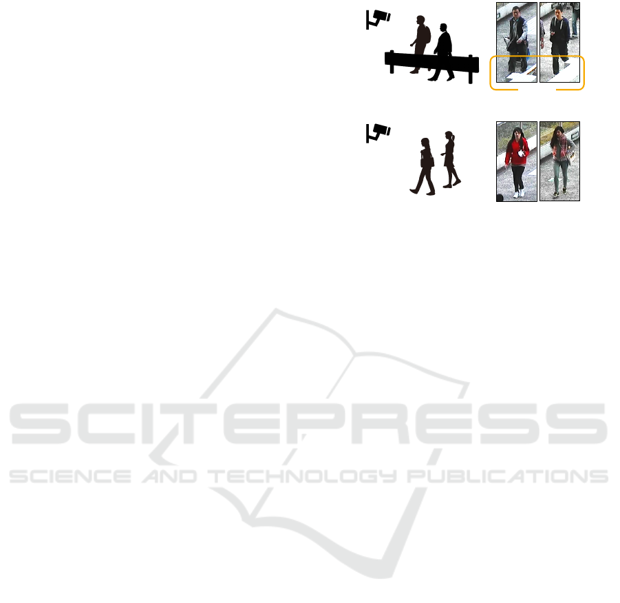
Here, we discuss a case whereby the training sam-
ples showing males contain a fence in the background
while the training samples showing females do not,
as shown in Figure 1. This case may be prevalent
Female
Male
Fence
Figure 1: Examples of training samples containing a bias
from the background surrounding the pedestrians.
when many females appear in the vicinity of a cer-
tain camera (e.g., near a cosmetics counter), and many
males appear in the vicinity of another camera (e.g.,
around a menswear section). In our preliminary ex-
periments, we observed that the accuracy of gender
classification declined when using training samples
containing a background bias (e.g., the presence or
absence of a fence). A random forest gender clas-
sifier included the background bias as discriminative
features rather than the true differences between the
physical appearances. For example, a test sample of a
female with a fence in front was incorrectly classified
as male. Avoiding this problem generally requires a
large number of training samples containing various
backgrounds for both genders. When the background
is obviously biased, we could modify the pedestrian
image collection strategy. In some cases, once the
sample collection is already complete, an unexpected
bias may be found in the training samples according
to the outputs of a gender classifier. Because the col-
lection of training samples is very time-consuming,
we may need to use the collected training samples
despite their bias. Therefore, our method aims to cor-
rectly classify gender using a weighted random fo-
rest incorporating a gaze distribution when the trai-
ning samples contain a background bias.
3 WEIGHTED RANDOM FOREST
USING A GAZE DISTRIBUTION
3.1 Overview of Decision Tree
Generation
The existing method for generating a random fo-
rest (Breiman, 2001) is as follows. Subsets of trai-
VISAPP 2019 - 14th International Conference on Computer Vision Theory and Applications
274

ning samples are prepared using bootstrap sampling,
and each subset is used to generate a decision tree in
the random forest. We denote a pixel of color c
i
in the
position (x
i
, y
i
) of a pedestrian image as a feature va-
lue f
i
(x
i
, y
i
, c
i
). In the field of computer vision (Gall
et al., 2011), the difference between pixel values in
an image observed from two positions is widely used
as a feature value. In this paper, we directly use the
pixel values as features to simplify the generation of
the decision trees in the random forest.
When generating each decision tree from each
subset of training samples, a feature value f
i
(x
i
, y
i
, c
i
)
and a threshold t
j
are randomly selected. The infor-
mation gain is computed using the selected feature va-
lue and selected threshold. The random selection of
f
i
(x
i
, y
i
, c
i
) and t
j
is repeated until M feature values
and N thresholds are stored. The stored feature values
and thresholds are used to determine a branch condi-
tion, where a training sample in a parent node is bran-
ched to either the left or right child node. The existing
method searches a branch condition using the infor-
mation gains computed from the candidate parame-
ters {x
i
, y
i
, c
i
, t
j
}. An information gain I
i, j
(x
i
, y
i
, c
i
, t
j
)
of a candidate parameter is represented as:
I
i, j
(x
i
, y
i
, c
i
, t
j
) = H(S) −
∑
k∈{L,R}
|S
k
|
|S|
H(S
k
), (1)
where S is a set of training samples in a parent node,
S
k
is a set of training samples in a child node, and H( )
is the entropy. Note that S
L
∩ S
R
= φ and S
L
∪ S
R
= S.
The branch condition at each node is represented as:

s ∈ S
L
f (x
i
, y
i
, c
i
) ≥ t
j
,
s ∈ S
R
otherwise.
Entropy is computed as follows:
H(S) = −
∑
a∈{male, f emale}
p(a)log(p(a)), (2)
where p(a) is the ratio of the training samples of gen-
der type a contained in the set S. The candidate pa-
rameter set corresponding to the maximum informa-
tion gain is used as a branch condition from the parent
node to the child nodes. The branch condition search
is repeated until the depth reaches a preset value.
3.2 Gaze Map
We represent the gaze distribution using the gaze map
described in (Nishiyama et al., 2018). To generate
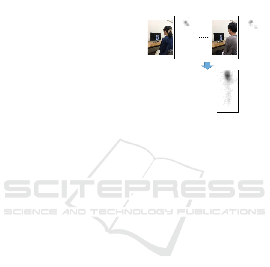
a gaze map, observers complete a pedestrian gender
classification task on stimulus images, and the ob-
server gaze locations are recorded. The average of
the measured gaze locations is computed across diffe-
rent observers and stimulus images. g(x
i
, y
i
) denotes a
Observer A Observer Z
1. Measure gaze distributions from observers 
determining pedestrian gender from stimulus images
2. Compute the average of 
the gaze distributions 
across the observers and
stimulus images.
Average
gaze map
Figure 2: Generating a gaze map from a gender classifica-
tion task assigned to oberservers.
pixel value at a position (x
i
, y
i
) of the gaze map. The
range of g(x
i
, y
i
) is set to [0, 1], and the size of the
gaze map is equal to that of the stimulus images. Fi-
gure 2 shows an overview of the process of generating
a gaze map from a gender classification task assigned
to multiple observers. In the figure, the dark region
in the gaze map represents the most frequent gaze lo-
cations gathered from the observers. Nishiyama et al.
demonstrated that the head region was the most pre-
valent gaze location when judging gender from pede-
strian images.
3.3 Assigning Weights for Feature
Selection
We describe the method of assigning weights for fea-
ture selection when generating a random forest. We
begin by outlining the existing methods (Breiman,
2001; Maudes et al., 2012). When applying the ex-
isting methods for gender classification, the position
(x
i
, y
i
) of a feature value is randomly selected accor-
ding to the uniform distribution. In contrast, our met-
hod selects the position (x
i
, y
i
) of a feature value ac-
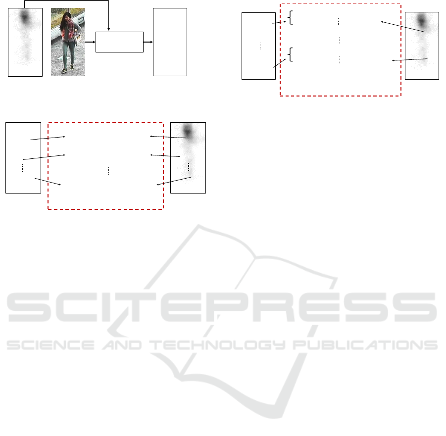
cording to the gaze distribution where a large weight
indicates the areas where the gaze locations of the ob-
servers are gathered. Figure 3 shows an overview of
our method. The figure demonstrates that the feature
values in the dark regions of g(x
i
, y
i
) (where the gaze
locations of observers are gathered) are frequently se-
lected.
Weighted Random Forest using Gaze Distributions Measured from Observers for Gender Classification
275

Gaze%map%
Pedestrian%
image%
×
×
×
×
×
Locations%of%
selected%features%
Weight%
Feature%
selection%
Figure 3: Assigning weights for feature selection.
×
×
Gaze map
Locations
of features
WeightsFeatures
(𝑥
1
, 𝑦
1
)
(𝑥
𝑀
, 𝑦
𝑀
)
𝑓
1
(𝑥
1
, 𝑦
1
, 𝑐
1
)𝑔(𝑥
1
, 𝑦
1
)
𝑓
2
(𝑥
2
, 𝑦
2
, 𝑐
2
)𝑔(𝑥
2
, 𝑦
2
)
𝑓
𝑀
(𝑥
𝑀
, 𝑦
𝑀
, 𝑐
𝑀
)𝑔(𝑥
𝑀
, 𝑦
𝑀
)
×
(𝑥
2
, 𝑦
2
)
×
×
×
Figure 4: Assigning weights for feature values.
3.4 Assigning Weights for Feature
Values
We describe a method for assigning weights for fea-
ture values when generating the random forest. The
existing methods (Breiman, 2001; Maudes et al.,
2012) did not modify the feature values. Maudes et
al. assigned random weights to the feature values ac-
cording to the uniform distribution. In contrast, our
method assigns weights according to the gaze distri-
bution represented as a gaze map g(x
i
, y
i
) using the
following equation:
f
0
(x
i
, y
i
, c
i
) = f (x
i
, y
i
, c
i
)g(x
i
, y
i
). (3)
Figure 4 shows an overview of our method. In the
figure, a weighted feature at position (x
i
, y
i
) attains a
large weight when it corresponds to the dark region
of g(x
i
, y
i
) where the gaze locations of the observers
are gathered. Note that the above procedure achieves
the same effectiveness as the preprocessing technique
described in (Nishiyama et al., 2018).
3.5 Assigning Weights for Information
Gains
We describe a method to assign weights for the infor-
mation gains when generating a random forest. We
explain our method by contrasting with the existing
methods (Breiman, 2001; Maudes et al., 2012). Brei-
man computed an information gain from parameter
candidates {x
i
, y
i
, c
i
, t
j
} as described in Section 3.1.
Maudes et al. computed information gains using the
same approach as Breiman and additionally weighted
×
×
Gaze map
Weights
Information gains of
candidates
(𝑥
1
, 𝑦
1
)
(𝑥
𝑀
, 𝑦
𝑀
)
𝐼
1,1
(𝑥
1
, 𝑦
1
, 𝑐
1
, 𝑡
1
)𝑔(𝑥
1
, 𝑦
1
)
𝐼
1,𝑁
(𝑥
1
, 𝑦
1
, 𝑐
1
, 𝑡
𝑁
)𝑔(𝑥
1
, 𝑦
1
)
𝐼
𝑀,1
(𝑥
𝑀
, 𝑦
𝑀
, 𝑐
𝑀
, 𝑡
1
)𝑔(𝑥
𝑀
, 𝑦
𝑀
)
𝐼
𝑀,𝑁
(𝑥
𝑀
, 𝑦
𝑀
, 𝑐
𝑀
, 𝑡
𝑁
)𝑔(𝑥
𝑀
, 𝑦
𝑀
)
×
×
Locations
of features
Figure 5: Assigning weights for information gains.
them according to the uniform distribution. In con-
trast, our method assigns weights for an information
gain according to the gaze distribution represented by
a gaze map g(x
i
, y
i
) using the following equation:
I
0
i, j
(x
i
, y
i
, c
i
, t
j
) = I
i, j
(x
i
, y
i
, c
i
, t
j
)g(x
i
, y
i
). (4)
We use the parameter set {x
i
, y
i
, c
i
, t
j
} that cor-
responds to the maximum information gain
I
0
max
(x
i
, y
i
, c
i
, t
j
) as a branch condition from a parent
node to a child node. Figure 5 shows an overview
of our method. In the figure, a weighted information
gain attains a large value when it corresponds to the
dark region of the gaze map g(x
i
, y
i
) where the gaze
locations of the observers are gathered.
4 EXPERIMENTS
4.1 Dataset
We evaluated the accuracy of our method on the
CUHK dataset included in the PETA dataset (Deng
et al., 2014). We used pedestrian images with or wit-
hout a bias created by a fence in the background sur-
rounding the pedestrians. We included training sam-
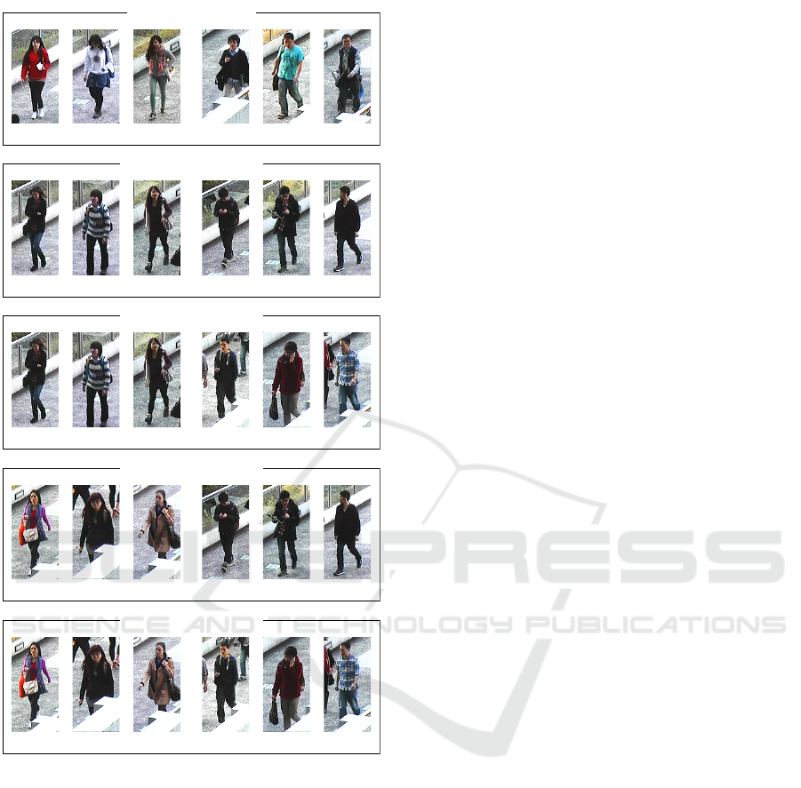
ples according to the following condition:
• T (Female, Male with a fence),
and test samples according to the following conditi-
ons:
• P1 (Female, Male),
• P2 (Female, Male with a fence),
• P3 (Female with a fence, Male),
• P4 (Female with a fence, Male with a fence).
Figure 6 shows examples of the training samples and
the test samples. The CUHK dataset consisted of 476
males without a fence, 426 males with a fence, 419 fe-
males without a fence, and 355 females with a fence.
The size of the pedestrian images was 80 ×160 pixels.
We used the gaze map shown at the bottom of Fi-
gure 2. We generated the gaze map using the pro-
cedure described in (Nishiyama et al., 2018). We
VISAPP 2019 - 14th International Conference on Computer Vision Theory and Applications
276

Male, fenceFemale
Training samples (T)
Test samples (P1)
Female Male
Test samples (P2)
Female Male, fence
Test samples (P3)
Female, fence Male
Test samples (P4)
Female, fence Male, fence
Figure 6: Examples of training samples T and test samples
P1 to P4 for gender classification.
used eight stimulus pedestrian images to measure the
gaze distribution from 14 observers. The stimulus
pedestrian images were randomly selected from the
CUHK dataset and were not included in either the
training samples or the test samples.
4.2 Basic Gender Classification
Performance
We evaluated the gender classification accuracy of the
following methods:
• Baseline (Breiman, 2001),
• Random weight (Maudes et al., 2012),
• Our method 1 (Assigning weights for feature se-
lection),
• Our method 2 (Assigning weights for feature va-
lues),
• Our method 3 (Assigning weights for information
gains).
We generated five test sets by randomly selecting
samples from the CUHK dataset. Each training set
consisted of 323 males and 323 females, and each test
set consisted of 17 males and 17 females. We set the
number of random selections for the feature values
to M = 196, the number of random selections for the
thresholds to N = 50, the number of decision trees to
200, and the depth of each decision tree to 5.
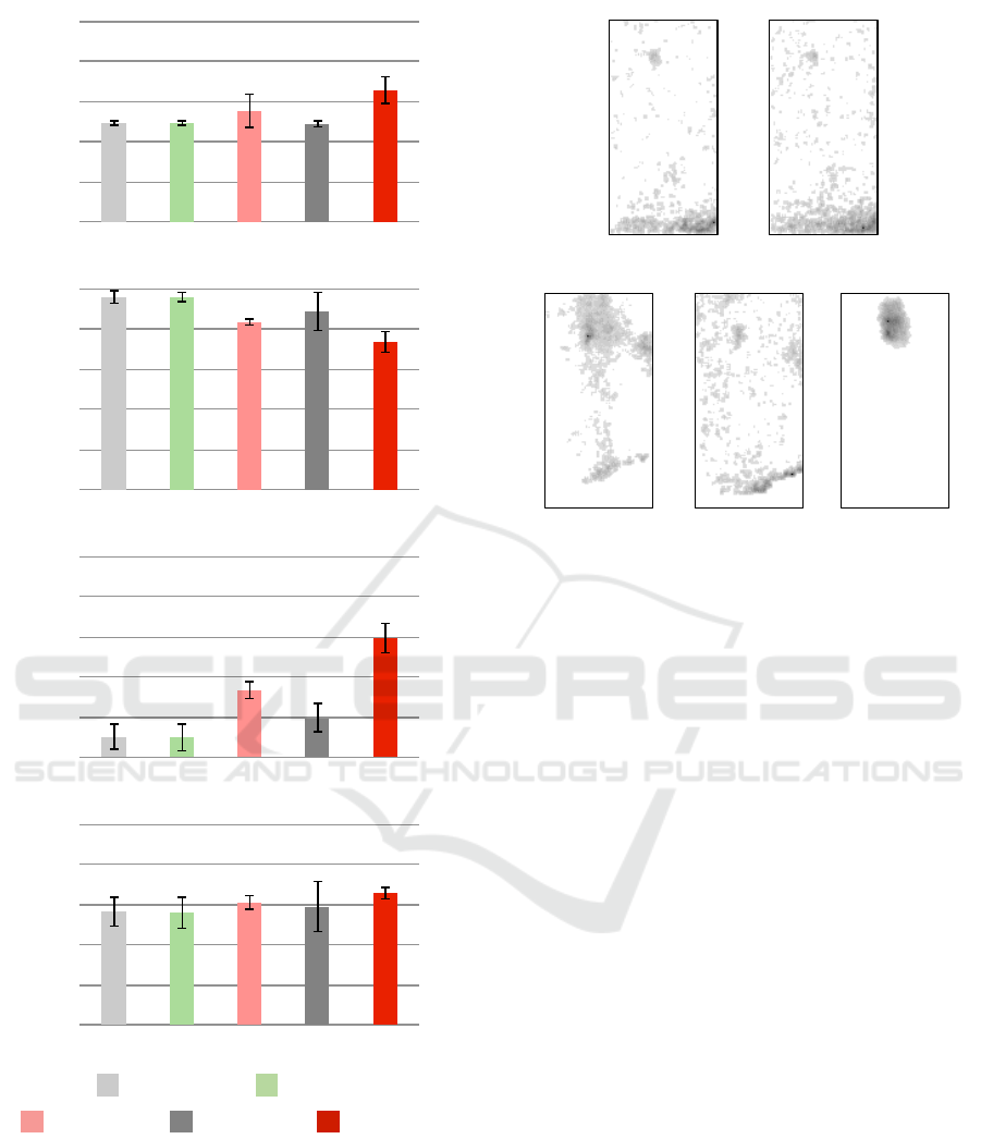
Figure 7 shows the accuracy of the gender classi-
fication for the training sample sets P1 to P4. We see
that the accuracies of the baseline and random weight
methods were almost the same for (a) to (d). Our met-
hods improve the accuracy for the scenarios where the
background differed between the training samples and
test samples, for (a), (c), and (d). In particular, assig-
ning weights for the information gain (our method 3)
outperformed the other methods for these scenarios.
However, our methods degraded the accuracy for (b).
To investigate the reason for the degradation, we con-
ducted a comparison using importance maps in the
next section.
4.3 Importance Map of the Random
Forest
We generated an importance map using the following
procedure:
1. We initialized an importance map of the same size
as the training samples and set each pixel value to
0.
2. We generated validation samples (out-of-bag) that
were not selected as training samples using boot-
strap sampling to generate each decision tree.
3. We input the validation samples into each decision
tree.
4. We computed an information gain I
i, j
(x
i
, y
i
, c
i
, t
j
)
or I
0
i, j
(x
i
, y
i
, c
i
, t
j
) for each node that was visited
by each validation sample.
5. We added the information gain to the pixel value
at position (x
i
, y
i
) in the importance map. We also
added the same value to the eight-neighborhood
of (x
i
, y
i
).
6. We suppressed extremely large values by compu-
ting the square root of the added value at each po-
sition in the importance map.
Weighted Random Forest using Gaze Distributions Measured from Observers for Gender Classification
277

(a) P1
(b) P2
(c) P3
(d) P4
Our method 1
Baseline Random weight
Our method 2 Our method 3
0
100
0
100
0
100
0
100
Accuracy (%)
Accuracy (%)
Accuracy (%)
Accuracy (%)
Figure 7: Accuracy of gender classification for training
sample sets P1 to P4.
Note that we used the training samples corresponding
to condition T described in Section 4.1.
Figure 8 shows the importance maps correspon-
ding to the baseline, random weight, our method 1,
our method 2, and our method 3. In the figure, the
dark regions represent the areas that each decision
(b) Random weight(a) Baseline
(c) Our method 1 (d) Our method 2 (e) Our method 3
Figure 8: Comparison between the importance maps of the
existing methods and our methods.
tree in the random forest regarded as discriminative
features when classifying gender. In (a) and (b), we
see that the values in the importance map were high
where there was a fence in the background. This in-
dicates that the presence or absence of a fence was
used for classifying gender by the existing methods.
In Figure 8(d), we see that the values of the impor-
tance map generated using our method were high for
a part of the fence in the background. For this reason,
if the weights of the gaze map were even slightly lar-
ger than zero, the thresholds for the branch conditions
in the decision trees were searched in the small range
of the weighted values.
In Figure 8(c) and (e), we see that the values of the
importance maps corresponding to our methods were
high in the head regions where the observers looked
most when judging gender. Note that the values in (c)
were also high for the background around the right
shoulders. This indicates that the training samples of
the CUHK dataset contain a background bias in addi-
tion to the fence that we did not originally consider.
We confirm that our method avoids the problem of
the additional background bias by using the weights
according to the gaze distribution.
To investigate the similarity between the impor-
tance map and the gaze map, we evaluated the nor-
malized correlation coefficient. We obtained −0.04
for the baseline method, −0.06 for the random weight
method, 0.40 for our method 1, −0.02 for our method
2, and 0.76 for our method 3. We confirmed that the
VISAPP 2019 - 14th International Conference on Computer Vision Theory and Applications
278

(a) Whole body (b) Upper body (c) Head and shoulders
Figure 9: Pedestrian images with manually selected parts.
similarity between the importance map and the gaze
map is high when using our method 3 to assign weig-
hts for the information gains.
4.4 Comparison using Manually
Selected Body Regions
To confirm the effectiveness of using a gaze distribu-
tion to generate the random forest, we evaluated the
accuracy of our method by comparing it with the ex-
isting methods on manually selected body regions. As
described in (Li et al., 2013), using manually selected
body regions improved the accuracy over the direct
use of pedestrian images. We evaluated the methods
using the following body regions:
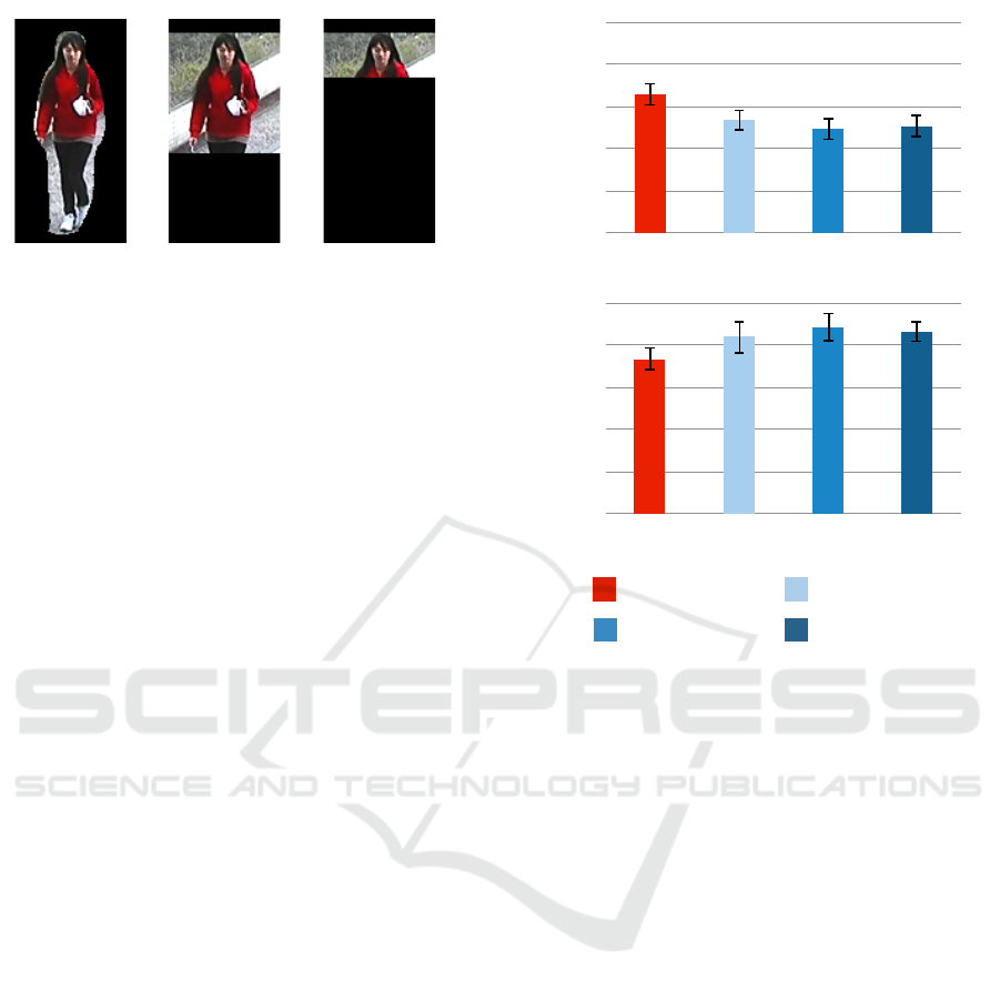
• Whole Body: We selected a region containing
the whole body by binarizing pixel values of the
average pedestrian image from the CUHK dataset.
Figure 9(a) shows an example of the whole body
region.
• Upper Body: We selected a region containing
the upper body according to the definitions of the
head, shoulders, and torso described in (Wu and
Nevatia, 2005). Figure 9(b) shows an example of
the upper body region.
• Head and Shoulders: We selected a region con-
taining the head and shoulders according to the
definition of the head and shoulders described
in (Wu and Nevatia, 2005). Figure 9(c) shows an
example of the head and shoulders region.
In the figure, the pixel values in the black region are
set to zero. We used the same regions for the trai-
ning samples and the test samples. We generated the
random forest using the baseline technique (Breiman,
2001). We used the same experimental conditions as
in Section 4.1, with the only difference being the body
region selection. For comparison, we use our method
3 (assigning weights for the information gain) that
acquired the highest accuracy in Section 4.2.
Figure 10 shows the accuracies of our method di-
rectly on the original images and the existing methods
(a) P1
(b) P2
Whole body
Head and shouldersUpper body
Our method 3
0
100
0
100
Accuracy (%)
Accuracy (%)
Figure 10: Accuracy of gender classification when using
manually selected image regions.
using manually selected body regions. We see that
our method outperformed the exisiting methods in (a).
However, the accuracy of our method was lower than
one of the existing methods in (b). To investigate the
degradation of the accuracy, we again generated im-
portance maps as described in Section 4.3. Figure 11
shows the importance maps of the existing methods
using manually selected body regions. In (a), the exis-
ting method using the whole body region emphasized
the presence of the fence at the feet of the pedestrians.
In (b) and (c), the existing methods using head, shoul-
der, and torso regions emphasized the background of
the right side of the pedestrians in addition to the head
regions. The accuracy of our method is superior to
that of the existing methods using manually selected
body regions because our method correctly ignores
the background bias as a feature for gender classifi-
cation.
5 CONCLUSION
We proposed a gender classification method using
gaze distribution to generate a random forest. Our
method assigned larger weights for feature selection,
feature values, and information gains corresponding
Weighted Random Forest using Gaze Distributions Measured from Observers for Gender Classification
279

(a) Whole body (b) Upper body (c) Head and
shoulders 
Figure 11: Comparison of importance maps when using
manually selected body parts.
to the predominant gaze locations of the observers.
We confirmed that our method significantly improved
the accuracy of gender classification in the presence
of a background bias.
In future work, we will further evaluate our met-
hod on various datasets using various human attribu-
tes. We will also explore the use of the gaze distribu-
tion with other machine learning techniques.
ACKNOWLEDGEMENTS
This work was partially supported by JSPS KA-
KENHI under grant number JP17K00238 and MIC
SCOPE under grant number 172308003.
REFERENCES
Amaratunga, D., Cabrera, J., and Lee, Y. S. (2008). Enri-
ched random forests. Bioinformatics, 24(18):2010 –
2014.
Antipov, G., Berrani, S., Ruchaud, N., and Dugelay, J.
(2015). Learned vs. hand-crafted features for pede-
strian gender recognition. In Proceedings of the 23rd
ACM International Conference on Multimedia, pages
1263–1266.
Breiman, L. (2001). Random forests. Machine learning,
45(1):5–32.
Deng, Y., Luo, P., Loy, C., and Tang, X. (2014). Pedestrian
attribute recognition at far distance. In Proceedings of
the 22nd ACM International Conference on Multime-
dia, pages 789–792.
Gall, J., Yao, A., Razavi, N., Gool, L. V., and Lempitsky, V.
(2011). Hough forests for object detection, tracking,
and action recognition. IEEE Transactions on Pat-
tern Analysis and Machine Intelligence, 33(11):2188–
2202.
Li, M., Bao, S., Dong, W., Wang, Y., and Su, Z. (2013).
Head-shoulder based gender recognition. In Pro-
ceedings of IEEE International Conference on Image
Processing, pages 2753–2756.
Maudes, J., Rodr
´
ıguez, J. J., Garc
´
ıa-Osorio, C., and Garc
´
ıa-
Pedrajas, N. (2012). Random feature weights for deci-
sion tree ensemble construction. Information Fusion,
13(1):20 – 30.
Murrugarra-Llerena, N. and Kovashka, A. (2017). Learning
attributes from human gaze. In Proceedings of IEEE
Winter Conference on Applications of Computer Vi-
sion, pages 510–519.
Nishiyama, M., Matsumoto, R., Yoshimura, H., and Iwai,
Y. (2018). Extracting discriminative features using
task-oriented gaze maps measured from observers for
personal attribute classification. Pattern Recognition
Letters, 112:241 – 248.
Rokach, L. (2016). Decision forest: Twenty years of rese-
arch. Information Fusion, 27:111 – 125.
Sattar, H., Bulling, A., and Fritz, M. (2017). Predicting the
category and attributes of visual search targets using
deep gaze pooling. In Proceedings of IEEE Internati-
onal Conference on Computer Vision Workshops, pa-
ges 2740–2748.
Schumann, A. and Stiefelhagen, R. (2017). Per-
son re-identification by deep learning attribute-
complementary information. In Proceedings of the
IEEE Conference on Computer Vision and Pattern Re-
cognition Workshops, pages 1435–1443.
Winham, S. J., Freimuth, R. R., and Biernacka, J. M.
(2013). A weighted random forests approach to im-
prove predictive performance. Statistical Analysis and
Data Mining, 6(6):496–505.
Wu, B. and Nevatia, R. (2005). Detection of multiple, par-
tially occluded humans in a single image by bayesian
combination of edgelet part detectors. In Proceedings
of Tenth IEEE International Conference on Computer
Vision, volume 1, pages 90–97.
VISAPP 2019 - 14th International Conference on Computer Vision Theory and Applications
280