Bilateral Random Projection based High-speed Face and Expression
Recognition Method
Jieun Lee, Miran Heo and Yoonsik Choe
School of Electrical and Electronic Engineering, Yonsei University, Seoul, Korea
Keywords:
Face Recognition, Greedy Algorithm, Random Projection, Sparse-based Representation Classification.
Abstract:
Face and expression recognition problem can be converted into superposition of low-rank matrix and sparse
error matrix, which have the merits of robustness to occlusion and disguise. Low-rank matrix manifests
neutral facial image and sparse matrix captures emotional expression with respect to whole image. To separate
these matrices, the problem is formulated to minimize the nuclear norm and L
1
norm, then can be solved by
using a closed-form proximal operator which is called Singular Value Thresholding (SVD). However, this
conventional approach has high computational complexity since it requires computation of singular value
decomposition of large sized matrix at each iteration. In this paper, to reduce this computational burden, a
fast approximation method for SVT is proposed, utilizing a suitable low-rank matrix approximation involving
random projection. Basically, being associated with sampling, a low-rank matrix is modeled as bilateral
factorized matrices, then update these matrices with greedy manner. Experiments are conducted on publicly
available different dataset for face and expression recognition. Consequently, proposed algorithm results in the
improved recognition accuracy and also further speeding up the process of approximating low-rank matrix,
compared to the conventional SVT based approximation methods. The best recognition accuracy score of
98.1% in the JAFFE database is acquired with our method about 55 times faster than SVD based method.
1 INTRODUCTION
Over the past decades, face and expression recogni-
tion have been particularly influential in the field of
computer vision and pattern recognition. The more
basic trends have been based on Eigenfaces (Turk and
Pentland, 1991), Fisherfaces (Belhumeur et al., 1997)
and SVM (Support Vector Machine), which has ari-
sen since past two decades (Yang et al., 2011). These
common algorithms aim all to collect proper featu-
res from face images for recognition. Neither of these
works treats the corrupted training data, and thus their
recognition results are fragile to the presence of ab-
rupt noise such as occlusion and disguise in face ima-
ges (Wei et al., 2014). Despite a certain level of
accurate performances of conventional face recogni-
tion algorithms, practical challenge remain regarding
the dramatic variations of pose, expression and illu-
mination. In addition, extreme illumination change
such as shadows weakens the assumption of a low-
dimensional linear model and then acts as occlusion
for face appearance model. These points imply that
face recognition should be robust to various occlusi-
ons for stable performance (Ou et al., 2014). Neutral
face images of the same person lie on a low-rank sub-
space due to their high correlation properties, whe-
reas facial expression can be regarded as sparse non-
rigid deformation in the presence of arbitrary face re-
gions. Namely we can employ the low-rank struc-
ture for finding the redundancy in the neutral face
images since there exists the similarity between those
images. Therefore researches have begun to inves-
tigate the link between low-rank or sparse structure
and facial and expression recognition for high accu-
racy purpose (Georgakis et al., 2016). In the context
of optimization skills, most works are conducted by
an efficient Alternating Direction Method of Multi-
pliers (ADMM) algorithm (Bertsekas, 2014) mostly
at finding component structures. ADMM has the pro-
perties of strong optimality and practical convergence
speed even for the case the objective function is non-
smooth. However this method can not be extended to
handle large scale dataset due to its limitation of ite-
rative mechanism. Recently dictionary learning based
study (Wei et al., 2014) promotes structural incohe-
rence in order to improve discrimination ability. Also
Augmented Lagrange multipliers (ALM) (Lin et al.,
2010) as one of ADMM has been applied to solve this
Lee, J., Heo, M. and Choe, Y.
Bilateral Random Projection based High-speed Face and Expression Recognition Method.
DOI: 10.5220/0007346000990106
In Proceedings of the 14th International Joint Conference on Computer Vision, Imaging and Computer Graphics Theory and Applications (VISIGRAPP 2019), pages 99-106
ISBN: 978-989-758-354-4
Copyright
c
 2019 by SCITEPRESS – Science and Technology Publications, Lda. All rights reserved
99

standard low-rank problem. ADMM is mainly asso-
ciated with the calculation of Singular Value Thres-
holding (SVT) operator (Cai et al., 2010) involving
SVD calculation which is the majority of the com-
putational load. However even for this computational
limit, SVT is widely used for low-rank approximation
as following reasons.
Consider the singular value decomposition of a
matrix X ∈ R
m×n
of rank r
X = UΣV
∗
,Σ = diag

{
σ
i
}
1≤i≤r

, (1)
where U and V are respectively m ×r and n ×r ma-
trices with orthonormal columns, and the singular va-
lues σ
i
are positive. For each τ ≥ 0, the soft threshol-
ding operator D
r
is defined as follows:
D
r
(X) := UD
r
(Σ)V
∗
,D
r
(Σ) = diag

t
{
σ
i
−τ
}
+

,
(2)
where t
+
is the positive part of t, namely, t
+
=
max(0,t). In other words, this operator simply ap-
plies a soft-thresholding rule to the singular values of
X, effectively shrinking these towards zeros. In some
sense, this shrinkage operator is a straightforward ex-
tension of the soft-thresholding rule for scalars and
vectors. In particular, note that if many of the singu-
lar values of X are below the threshold τ, the rank of
D
r
(X) may be considerably lower than that of X, just
like the soft-thresholding rule applied to vectors leads
to sparser outputs whenever some entries of the input
are below threshold. The singular value thresholding
operator is the proximity operator associated with the
nuclear norm,
D
r
(Y ) = argmin
X

1
2
k
X −Y
k
2
F
+ τ
k
X
k
∗

. (3)
Eq. 3 is proved in Theorem 2.1 by (Cai et al., 2010)
in detail. Due to this powerful attributes, SVT is used
frequently but it has a complexity equal to that of
SVD, i.e., O(mn ·min(m,n)) at each iteration.
Therefore in order to solve the low-rank and
sparse decomposition with a gross error term, the
greedy bilateral scheme has been explored and ex-
ploited. This greedy scheme (Zhou and Tao, 2013)
uses only QR decompositions, random projections,
and matrix multiplications, thus, it reduces computa-
tional complexity very efficiently. In this paper, this
greedy method is adopted to predict the low-rank ma-
trix fast and a novel random projection based method
is proposed in order to reduce the computational bur-
den for low-rank approximation of classical facial re-
cognition framework.
2 RELATED WORK
In this section, we firstly mention a brief formulation
on face recognition based on (Georgakis et al., 2016).
Then the optimization skill for reducing computatio-
nal burden will be described in detail and the propo-
sed overall method will be finally introduced in the
next section.
2.0.1 Discriminant Incoherent Component
Analysis
The goal of DICA (Discriminant Incoherent Compo-
nent Analysis) (Georgakis et al., 2016) is to robus-
tly learn components from training samples that 1)
are discriminant and exhibit low-complexity structu-
res (e.g., low-rank or sparsity) associated with facial
attributes, 2) are mutually incoherent among different
classes, and 3) facilitate the classification of test sam-
ples by means of sparse representation. This method
learns the reconstruction matrices
n
U
(i)
o
n
c
i=1
and pro-
jection matrices
n
V
(i)
o
n
c
i=1
by employing the training
matrix X ∈ R
d×N
which contains in its columns the
vectorized training face images, with d being the di-
mensionality of each image and N the number of trai-
ning observations. Also n
c
denotes the total number
of each class. The column of X, x represents a vec-
torized expressive face image. According to DICA
algorithm, we can formulate the face and expression
recognition problem as folowing:
argmin
W
λ
(i)
n
c
∑
i=1



V
(i)



(·)
+ η
∑
i6= j



V
(i)
V
( j)
T



2
F
+ λ
1
k
O
k
1
,
s.t. X =
n
c
∑
i=1
U
(i)
V
(i)
X +O,
U
(i)
T
U
(i)
= I, i = 1, 2,...,n
c
.
(4)
In Eq. 4, the set W is comprised of three compo-
nents U
(i)
, V
(i)
and O. Furthermore the structure-
inducing norm



V
(i)



(·)
is either the nuclear norm for
face-specific projections or the l
1
-norm for expession-
specific projections. The term
∑
i6= j



V
(i)
V
( j)
T



2
F
in-
duces mutual incoherence among the projection spa-
ces and O ∈ R
d×N
denotes the outlier matrix accoun-
ting for components that cannot be explained by the
summand containing the class-specific reconstructi-
ons. The positive parameters λ
(i)
, η, and λ
1
control
the norm imposed on
n
V
(i)
o
n
c
i=1
, the mutual incohe-
rence for all component pairs, and the sparsity of out-
VISAPP 2019 - 14th International Conference on Computer Vision Theory and Applications
100

liers O, respectively. The orthonormality is endowed
wih U
(i)
in order to characterize each class properly.
2.0.2 Optimization
Previously, the Alternating-Directions Method of
Multipliers (ADMM) (Bertsekas, 2014) is employed
to solve Eq. 4. This utilizes the partial augmen-
ted Lagrangian function for Eq. 4. At each itera-
tion, the Lagrangian function is minimized with re-
spect to each variable in W in an alternating fashion.
Subsequently the Lagrange multiplier and parameter
are updated too. When the nuclear norm is enfor-
ced on V
(i)
, the cost of each iteration is mainly as-
sociated with the calculation of the SVT. Hence com-
putational complexity about V
(i)
update amounts to
O

max

d
2
N,dN
2

.
Note that the optimization equation for V can be
expressed as follows
argmin
V
(i)
L(V
(i)
,Y [t],µ[t])
= argmin
V
(i)
λ
(i)



V
(i)



∗
+ η
∑
i6= j



V
(i)
V
( j)
T



2
F
+
µ[t]
2





X −
n
c
∑
i=1
U
(i)
V
(i)
X −O + µ[t]
−1
Y [t]





2
F
= argmin
V
(i)
λ
(i)



V
(i)



∗
+ f (V
(i)
)
(5)
where µ is a positive parameter and Y ∈ R
d×N
is the
Lagrange multiplier related to the linear constraint.
Eq. 5 consists of a non-smooth term, induced by the
nuclear norm, and a smooth, twice differentiable term
described by the function f . It can easily be proved
that the gradient ∇ f is Lipschitz-continuous. By li-
nearizing f in the vicinity of the current point V
(i)
[t],
and by exploiting the Lipschitz-continuity of ∇ f , we
obtain the following equivalent problem
argmin
V
(i)
λ
(i)



V
(i)



∗
+
1
2




V
(i)
−(V
(i)
[t] −
1
L
∇ f (V
(i)
[t]))




2
F
(6)
where L is the Lipschitz constant. Instead of applying
the SVT operator, we choose greedy bilateral method
for Eq. 6.
The heart of our SVD-free method shares the idea
of Zhou et al. (Zhou and Tao, 2013), in that the above
equation can be found by applying greedy bilateral
projection to matrix instead of the original SVT-based
method as illustrated in (Georgakis et al., 2016).
3 PROPOSED METHOD
Greedy strategy has strength when it is used as warm
start of the next higher rank optimization and speeds
up convergence since it is robust to biased rank esti-
mation. In addition, its mutually adaptive updates of
two factors which comprise the target matrix yields a
simple yet efficient SVD-free implementation. Gene-
rally under this technique, the overall time complex-
ity of matrix completion is only dependent on rank of
the target matrix. In real world application, finding
the exact low-rank matrix is intractable. There ex-
ists trade-off between accuracy and time/space costs,
even if singular values of the target matrix decay fast.
Although the low-rank matrix approximation in Eq. 6
is provably optimal when constructed from SVD, the
expensive time cost makes SVT prohibitive to large
matrix. Therefore this type of problem can be resol-
ved by designing a suitable random projection matrix
with greedy manner.
In this paper, we adopt two main algorithms by
mitigating computational complexity compared to the
SVT-based algorithm like DICA (Georgakis et al.,
2016).
3.0.1 Greedy Bilateral Method (GBM)
To apply this method, we slightly change the problem
of Eq. 6 in terms of UV factors based on the assump-
tion of low-rank constraint on F
min
U,V
k
F −UV
k
2
F
, s.t. rank(U) = rank(V ) ≤ r, (7)
where F = V
(i)
−

V
(i)
[t] −
1
L
∇ f (V
(i)
[t])

. In U, V in
Eq. 7 are different from the aboved mentioned recon-
struction and projection matrices. Alternatively op-
timizing U and V in Eq. 7 immediately yields the
following updating rules, note subscript in ·
k
denotes
the variable in the k
th
iterate and (·)
†
stands for the
Moore-Penrose pseudo-inverse:
(
U
k
= FV
T
k−1

V
k−1
V
T
k−1

†
V
k
=

U
T
k
U
k

†
U
T
k
F.
(8)
It can be observed that the object value in Eq. 7 is
merely determined by the matrix product UV rather
than individual U or V , and different (U,V ) pair can
produce the same UV . It is then of interest to find a
pair of (U,V ) that have the same product as (U
k
,V
k
)
in Eq. 8 but can be computed in less time than U
k
and
V
k
. This observation is represented by investigating
the product U
k
V
k
,
U
k
V
k
= U
k

U
T
k
U
k

†
U
T
k
F = P
U
k
F. (9)
Bilateral Random Projection based High-speed Face and Expression Recognition Method
101

This implies that the product U
k
V
k
equals to the ort-
hogonal projection of F onto the column space of U
k
.
According to Eq. 8, the column space of U
k
can be
represented by arbitrary orthonormal basis for the co-
lumns of FV
T
k−1
.
It is worth noting that we can compute it as Q via
fast QR decomposition FV
T
k−1
= QR. In this case,
the product U
k
V
k
can be equivalently computed as
U
k
V
k
= P
Q
F = QQ
T
F. Therefore U
k
and V
k
in Eq.
8 can be replaced by Q and Q
T
F repsectively, while
the product U
k
V
k
and the corresponding object value
are kept the same. This gives a faster updating proce-
dure
(
U
k
= Q, QR = qr(FV
T
k−1
)
V
k
= Q
T
F.
(10)
This relation can then be derived, from which the
alternating update can be viewed as mutually adap-
tive optimization of right sketch FV
T
and left ske-
tch Q
T
F for F. Since the right and left sketches re-
spectively describe the column and row spaces, which
largely decide the approximation precision, we can
temporarily ignore the QR decomposition in order to
see how the column/row space is tracked within this
scheme. Actually Eq. 8 has the same accuracy as po-
wer scheme randomized SVD method (Halko et al.,
2011). Different from power scheme, we updates Eq.
8 with a greedy incremental rank for both U and V .
The computatioin of GBM is dominated by the two
matrix multiplications that take 2dNr
i
flops. It can be
further speeded up if assigning sparsity on U and V ,
which will be described in the next subsection. The
overall greedy bilateral solver is wrapped up in Algo-
rithm 1.
3.0.2 Random Row-Space Projection (RRSP)
Beyond greedy bilateral method, in this section we
outline a scheme that is based on the approximate
SVD algorithm of Sarlos (Sarlos, 2006), (Fazel et al.,
2008). This method casts SVD-free algorithm as a di-
rect sensing the row and column space of the target
matrix.
Suppose rank(F) = r, we again perform two sets
of measurements (arbitrary random matrix) of F.
Here, the output of the first set is used as the sensing
matrix for the second set. Thus this method needs to
access F and F
T
to obtain the two sets of measure-
ments sequentially. The second set of measurements
are in fact quadratic in F.
We again have several choices for the sensing ma-
trix P ∈ R
r×m
, for example we can pick P with i.i.d.
Gaussian entries. It is also possible to use structu-
red matrices that are faster to apply, for example the
SRFT (The Subsampled Randomized Fourier Trans-
form) matrix which consists of randomly selected
rows of the product of a discrete Fourier transform
matrix and a random diagonal matrix (Woolfe et al.,
2008). From the viewpoint of sparsity, SRFT matrix
is encouraged to be the sensing matrix P. We can con-
sider the following scheme:
• Sensing : Make linear measurement
Y
1
= PF, f ollowed by Y
2
= Y
1
F
T
. (11)
• Recovery : Given measurements Y
1,2
, construct
ˆ
F
T
= Y
†
1
Y
2
(12)
The recovery step can be implemented eifficiently
using a QR decomposition of Y
1
.
A geometric interpretation is as follows: using
ˆ
F
T
= Y
†
1
Y
1
F
T
= (PF)
†
(PF) F
T
and noting that Y
†
1
Y
1
is the orthogonal projection matrix onto the range of
Y
1
, we see that the estimate
ˆ
F is given by the pro-
jection of each row of F onto the row-space of PF,
which is spanned by random linear combinations of
the rows of F. That is, each row of F is approxi-
mated by its closest vector in the row-space of PF.
Employing random projection matrix P is of crucial
importance in extracting informative spaces from the
target matrix and determining the effective rank. The
methodology presented in this work is verified by the
following Lemma 1.
Lemma 3.1. (Exact Recovery) Suppose entries of P
are i.i.d. Gaussian.
If rank(F) = r, the scheme described in Eq. 11 and
12 yields
ˆ
F = F with probability one.
Proof. Let p
i
denote the ith row or P (for example,
from a Gaussian or SRFT ensemble). If rank(F) = r
the set of random vectors F
T
p
i
, i = 1,..., r are linearly
independent with probability one, which implies that
row-space of PF is equal to row-space of F with pro-
bability one, and projecting F onto its own row-space
gives F.
To cope with relative error of SRFT matrix used,
the proof is in section 5.2 (Woolfe et al., 2008).
Lemma 3.2. Suppose P is an SRFT matrix and there
are α, β > 1 such that
α
2
β
(α −1)
2

2r
2

≤ l < m (13)
Then,


ˆ
F −F


= C
√
m ·σ
r+1
(F) (14)
holds with probability at least 1 −
1
β
. Constant C de-
pends on α.
However when F is not low-rank structure, the
truncated r-term SVD of F is approximated by

Y
†
1
Y
2

r
.
VISAPP 2019 - 14th International Conference on Computer Vision Theory and Applications
102

Table 1: Recognition Rates (%) For Subject-Independent Face & Expression Recognition (SIR) on CK+ Dataset (Lucey
et al., 2010).
Method Image Size (pixel)
SIR
Time (Sec)
Face Expression
DICA
32 × 32 5.5556 61.2903 4.3052·10
3
/ 3.4130 ·10
3
48 × 48 5.5556 79.6296 1.7219·10
3
/ 1.8398·10
3
56 × 56 5.5556 78.7037 1.6105·10
4
/1.4448·10
4
BGM
32 × 32 27.7778 61.2903 7.5450 / 6.1080
48 × 48 41.6667 68.5185 23.1306 / 25.1301
56 × 56 42.5926 69.4444 141.3831 / 125.3712
RRSP [Gaussian]
32 × 32 45.3704 72.2222 7.3872 / 8.8441
48 × 48 47.2222 73.1481 21.3828 / 25.57
56 × 56 52.7778 74.0741 134.2379 / 123.5661
RRSP [SRFT]
32 × 32 78.7037 35.1852 9.5474 / 6.7210
48 × 48 81.4815 42.5926 21.4391 / 21.5486
56 × 56 78.7037 49.0741 132.4659 / 119.2481
Table 2: Recognition Rates (%) For Subject-Independent Face & Expression Recognition (SIR) on The Japanese Female
Facial Expression (JAFFE) Database (Lyons et al., 1998).
Method Image Size (pixel)
SIR
Time (Sec)
Face Expression
DICA
32 × 32 8.3333 40.6250 1.3333·10
3
/ 1.3565 ·10
3
48 × 48 4.1667 42.1875 1.418·10
3
/ 1.7989·10
3
56 × 56 4.1667 42.1875 6.3770·10
3
/ 1.9214·10
4
BRM
32 × 32 75 48.4375 5.3755 / 11.8196
48 × 48 75 50 10.6103 / 10.4784
56 × 56 50 48.4375 136.8656 / 114.6812
RRSP [Gaussian]
32 × 32 75 48.4375 5.5414 / 7.2722
48 × 48 62.5 48.4375 10.5549 / 12.2985
56 × 56 79.1667 50 107.6488 / 124.2132
RRSP [SRFT]
32 × 32 98.1 32.8125 5.5350 / 6.1037
48 × 48 98.1 28.1250 11.86 / 10.9866
56 × 56 98.1 35.9375 114.9448 / 127.9194
Table 3: Recognition Rates (%) For Subject-Independent Face & Expression Recognition (SIR) on The Yale Face Database
B (Belhumeur et al., 1997).
Method Image Size (pixel)
SIR
Time (Sec)
Face Expression
DICA
32 × 32 34.2857 33.3333 337.7671 / 194.3378
48 × 48 31.4286 33.3333 700.5026 / 350.008
56 × 56 31.4286 40 7.1175·10
3
/ 3.8683·10
3
BGM
32 × 32 60 46.6667 9.5883 / 5.7042
48 × 48 42.8571 43.3333 21.2742 / 9.8354
56 × 56 60 36.6667 201.1026 / 101.0096
RRSP [Gaussian]
32 × 32 74.2857 36.6667 10.5794 / 5.7042
48 × 48 82.8571 43.3333 21.3447 / 9.8354
56 × 56 82.8571 36.6667 196.1838 / 105.8419
RRSP [SRFT]
32 × 32 80 33.3333 10.1339 / 6.5179
48 × 48 82.8571 43.3333 24.1405 / 10.3150
56 × 56 71.4286 43.3333 205.8391 / 103.4070
Bilateral Random Projection based High-speed Face and Expression Recognition Method
103

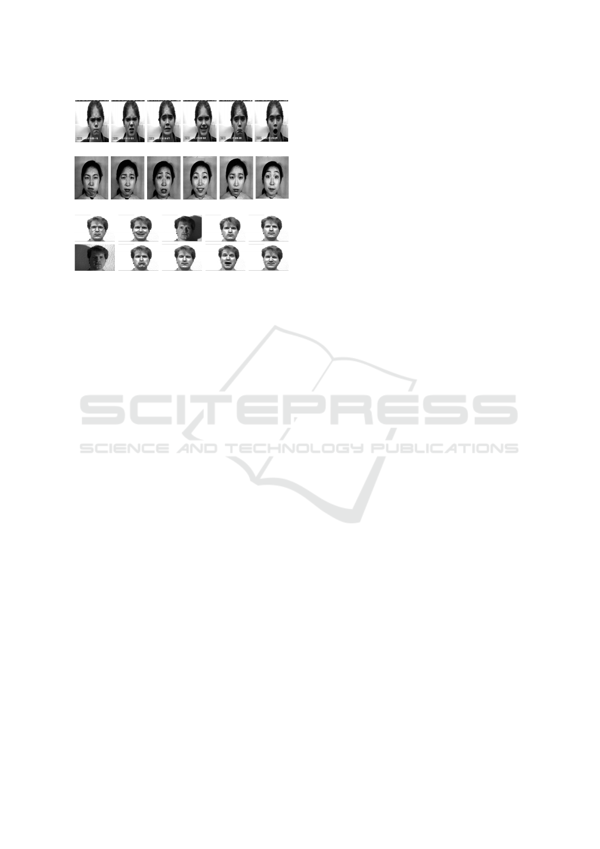
(a)
(b)
(c)
Figure 1: Example images from each of the datasets used.
(a) CK+ (Lucey et al., 2010). (b) The Japanese Female Fa-
cial Expression (JAFFE) Database (Lyons et al., 1998). (c)
The Yale Face Database B (Belhumeur et al., 1997).
4 EXPERIMENTAL RESULTS
In this section, the effectiveness of our random pro-
jection based approach is verified through a number of
experiments. Our method explores concrete applica-
tion, face and expression recognition on CK+, JAFFE
and The Yale Face Database B dataset. The experi-
mental setting is identical to that of DICA algorithm
(Georgakis et al., 2016). Specifically, training and test
dataset for expression recognition is comprised of the
six universal emotions (Anger, Disgust, Fear, Happi-
ness, Sadness and Surprise).
CK+ has been widely used for the task of face and
expression recognition. It contains 123 subjects in a
total of 593 sequences, 327 out of which are annotated
with respect to the emotion portrayed. We does not
consider the temporal dimension, only the last 4 fra-
mes are used as expressive images, as those are close
to the apex phase of the expression. JAFFE database
contains 213 images of 6 basic facial expressions po-
sed by 10 Japanese female models. Each image has
been rated on 6 emotion adjectives by 60 Japanese
subjects. The Yale Face Database B database con-
tains 5760 single light source images of 10 subjects
each seen under 576 viewing conditions. For every
subject in a particular pose, an image with ambient
background illumination was captured. We randomly
extract the number of training subjects 25, 10 and 15
for CK+, JAFFE and Yale Face Database B respecti-
vely.
Addtionally, to examine how dimensionality of
the image affects accuracy, the following experiments
Tab. 1, 2, and 3 are conducted. Only the choice of
48×48, 56 ×56 pixels for the image size of the DICA
algorithm (Georgakis et al., 2016) of CK+ Dataset le-
ads to the best performance. Except in that event, the
proposed methods achieve the best results and are si-
multaneously conducted with fast time. In face recog-
nition works, RRSP based on SRFT projection matrix
performs the best, primarily due to test images being
associated with sparse linear combinations of similar
faces rather than similar expressions in the dictionary.
We achieved the best performances on the JAFFE da-
taset because it consist of no dramatic illumination or
pose changes.
On average the computation time of DICA (Ge-
orgakis et al., 2016) is about 130.7098, 113.3263 and
35.6343 times higher than the random projection ba-
sed methods (i.e., Bilateral Greedy method, RRSPs)
in CK+, JAFFE and The Yale Face Database B, re-
spectively. This is due to the iterative steps of the
cost function in ADMM algorithm of DICA because
the shrinkage operator about L
1
norm becomes the
most time-consuming calculation, thus entailing li-
near complexity O(dN).
We remark that these experimental results are fe-
asible because the face and expression recognition
system does not need to restore the whole pixels of
the structured image with perfect accuracy. It clearly
shows that our method can handle data in large scale.
5 CONCLUSION
We propose a novel method for face and expres-
sion recognition that utilizes two simple and extensi-
ble random projection based optimization algorithms.
The proposed method updates two factors of target
matrix in ways of bilateral and direct projection met-
hods, maintaining the accuracy of extracting low-rank
matrix. In experiments, we compare our approach
with a SVD-based method through real-world exam-
ples. Experimental results depict that excellent face
and expression recognition results up to 98.1% can
be obtained with a surprisingly small amount of time
by 55 times smaller than SVD based method, such as
DICA.
ACKNOWLEDGEMENTS
This work was supported by the Technology In-
novation Program (or Industrial Strategic Techno-
logy Development Program(10073229, Development
of 4K high-resolution image based LSTM network
deep learning process pattern recognition algorithm
VISAPP 2019 - 14th International Conference on Computer Vision Theory and Applications
104

Algorithm 1: Greedy bilateral solver.
Input : Data X ∈ R
d×N
. Parameters : λ
(i)
,η, λ
1
, and
n
m
(i)
o
n
c
i=1
, Objective function f , rank step size ∆r,
power K.
Output:
n
U
(i)
∈ R
d×m
(i)
,V
(i)
∈ R
m
(i)
×d
o
n
c
i=1
,O ∈R
d×N
.
1 Normalize each column of X to unit l
2
-norm
2 Initialize : Set
nn
U
(i)
[0]
o
,
n
V
(i)
[0]
oo
n
c
i=1
, O[0],Y [0] to zero matrices. Set
µ[0] = 1/
k
X
k
,ρ = 1.1,µ
max
= 10
10
.
3 while not converged do
4 for i = 1 : n
c
do
5 Calculate L = 1.02λ
max
h
µ[t]XX
T
+ 2η
∑
i6= j
V
( j)
[t]
T
V
( j)
[t]
i
;
6 if V
(i)
is associated with nuclear norm then
7 for k ← K do
8 U
k
= Q, QR = qr(FV
T
k−1
) ;
9 V
k
= Q
T
F;
10 end
11 Calculate the top ∆r right singular vectors v (or ∆r-dimensional random projections) of
∂ f
∂V
;
12 Set V := [V ; v] ;
13 else if V
(i)
is associated with l
1
-norm then
14 V
(i)
[t + 1] ← S
λ
(i)
L
h
V
(i)
[t] −L
−1
∇ f (V
(i)
[t])
i
;
15 else
16 U
(i)
[t + 1] ← P
h
X −
∑
i6= j
U
( j)
[t]V
( j)
[t + 1]X −O[t] + µ[t]
−1
Y [t]

V
(i)
[t + 1]X
T
i
;
17 end
18 end
19 O[t + 1] ← S
λ
1
µ[t]
h
X −
∑
n
c
i=1
U
(i)
[t + 1]V
(i)
[t + 1]X + µ[t]
−1
Y [t]
i
;
20 Update the Lagrange multiplier by Y [t + 1] ←Y [t] + µ[t]

X −
∑
n
c
i=1
U
(i)
[t + 1]V
(i)
[t + 1]X −O[t + 1]

;
21 Update µ by µ[t + 1] = min(ρ ·µ[t], µ
max
) ;
22 end
for real-time parts assembling of industrial robot for
manufacturing) funded By the Ministry of Trade, In-
dustry & Energy(MOTIE, Korea)
REFERENCES
Belhumeur, P. N., Hespanha, J. P., and Kriegman, D. J.
(1997). Eigenfaces vs. fisherfaces: Recognition using
class specific linear projection. Technical report, Yale
University New Haven United States.
Bertsekas, D. P. (2014). Constrained optimization and La-
grange multiplier methods. Academic press.
Cai, J.-F., Cand
`
es, E. J., and Shen, Z. (2010). A singular
value thresholding algorithm for matrix completion.
SIAM Journal on Optimization, 20(4):1956–1982.
Fazel, M., Candes, E., Recht, B., and Parrilo, P. (2008).
Compressed sensing and robust recovery of low rank
matrices. In Signals, Systems and Computers, 2008
42nd Asilomar Conference on, pages 1043–1047.
IEEE.
Georgakis, C., Panagakis, Y., and Pantic, M. (2016). Dis-
criminant incoherent component analysis. IEEE tran-
sactions on image processing, 25(5):2021–2034.
Halko, N., Martinsson, P.-G., and Tropp, J. A. (2011). Fin-
ding structure with randomness: Probabilistic algo-
rithms for constructing approximate matrix decompo-
sitions. SIAM review, 53(2):217–288.
Lin, Z., Chen, M., and Ma, Y. (2010). The aug-
mented lagrange multiplier method for exact reco-
very of corrupted low-rank matrices. arXiv preprint
arXiv:1009.5055.
Lucey, P., Cohn, J. F., Kanade, T., Saragih, J., Ambadar,
Z., and Matthews, I. (2010). The extended cohn-
kanade dataset (ck+): A complete dataset for action
unit and emotion-specified expression. In Computer
Vision and Pattern Recognition Workshops (CVPRW),
2010 IEEE Computer Society Conference on, pages
94–101. IEEE.
Bilateral Random Projection based High-speed Face and Expression Recognition Method
105

Lyons, M., Akamatsu, S., Kamachi, M., and Gyoba, J.
(1998). Coding facial expressions with gabor wa-
velets. In Automatic Face and Gesture Recognition,
1998. Proceedings. Third IEEE International Confe-
rence on, pages 200–205. IEEE.
Ou, W., You, X., Tao, D., Zhang, P., Tang, Y., and Zhu, Z.
(2014). Robust face recognition via occlusion dictio-
nary learning. Pattern Recognition, 47(4):1559–1572.
Sarlos, T. (2006). Improved approximation algorithms for
large matrices via random projections. In Foundations
of Computer Science, 2006. FOCS’06. 47th Annual
IEEE Symposium on, pages 143–152. IEEE.
Turk, M. A. and Pentland, A. P. (1991). Face recognition
using eigenfaces. In Computer Vision and Pattern Re-
cognition, 1991. Proceedings CVPR’91., IEEE Com-
puter Society Conference on, pages 586–591. IEEE.
Wei, C.-P., Chen, C.-F., and Wang, Y.-C. F. (2014). Robust
face recognition with structurally incoherent low-rank
matrix decomposition. IEEE Transactions on Image
Processing, 23(8):3294–3307.
Woolfe, F., Liberty, E., Rokhlin, V., and Tygert, M. (2008).
A fast randomized algorithm for the approximation of
matrices. Applied and Computational Harmonic Ana-
lysis, 25(3):335–366.
Yang, M., Zhang, L., Yang, J., and Zhang, D. (2011). Ro-
bust sparse coding for face recognition. In Computer
Vision and Pattern Recognition (CVPR), 2011 IEEE
Conference on, pages 625–632. IEEE.
Zhou, T. and Tao, D. (2013). Greedy bilateral sketch, com-
pletion & smoothing. In International Conference on
Artificial Intelligence and Statistics. JMLR. org.
VISAPP 2019 - 14th International Conference on Computer Vision Theory and Applications
106