Polyp Classiﬁcation and Clustering from Endoscopic Images using

Competitive and Convolutional Neural Networks

Avish Kabra

, Yuji Iwahori

, Hiroyasu Usami

, M. K. Bhuyan

, Naotaka Ogasawara

and Kunio Kasugai

Indian Institute of Technology Guwahati, Assam, 781039, India

Chubu University, 487-8501, Japan

Aichi Medical University, 1-1 Yazakokarimata, Nagakute, Aichi, 480-1195, Japan

Keywords:

Competitive Learning, Deep Learning, Convolutional Neural Networks.

Abstract:

Understanding the type of Polyp present in the body plays an important role in medical diagnosis. This paper

proposes an approach to classify and cluster the polyp present in an Endoscopic scene into malignant or

benign class. CNN and Self Organizing Maps are used to classify and cluster from white light and Narrow

Band (NBI) Endoscopic Images . Using Competitive Neural Network different polyps available from previous

data are plotted with the new polyp according to their structural similarity. Such kind of presentation not only

help the doctor in it’s easy understanding but also helps him to know what kind of medical procedures were

followed in similar cases.

1 INTRODUCTION

According to the WHO, Cancer is the second lead-

ing cause of death globally, and is responsible for

an estimated 9.6 million deaths in 2018. Globally,

about 1 in 6 deaths is due to cancer . This report

veriﬁes that Late-stage presentation and inaccessi-

ble diagnosis and treatment are common reasons for

these deaths. In 2017, only 26 percent of low-income

countries reported having pathology services gener-

ally available in the public sector. More than 90 per-

cent of high-income countries reported treatment ser-

vices are available compared to less than 30 percent

of low-income countries.

This provides a vast area of research so that diag-

nosis can be made easy and accessible. Many meth-

ods have been developed to know the existence of a

polyp in an Endoscopic scene but the automatic clas-

siﬁcation of these into different classes is still com-

plex (Y.Iwahori and K.Kasugai, 2013). This paper

proposes a method to know whether the polyp de-

tected in a patient’s body is benign or malignant be-

cause the ﬁrst step after being diagnosed with a tumor

is to ﬁnd it’s class. In short, the meaning of malig-

nant is cancerous and the meaning of benign is non-

cancerous that is why it is very important to have a

proper veriﬁcation and to decide the further treatment

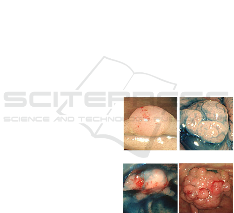
Figure 1: (i)White light Benign (ii)StainNBI Benign.

Figure 2: Malignant (i)StainNBI (ii)White Light.

path. A timely understanding of the tumor can prevent

deaths.

446

Kabra, A., Iwahori, Y., Usami, H., Bhuyan, M., Ogasawara, N. and Kasugai, K.

Polyp Classiﬁcation and Clustering from Endoscopic Images using Competitive and Convolutional Neural Networks.

DOI: 10.5220/0007353204460452

In Proceedings of the 8th International Conference on Pattern Recognition Applications and Methods (ICPRAM 2019), pages 446-452

ISBN: 978-989-758-351-3

2 LITERATURE SURVEY

Present methods of image clustering mostly involve

use of K-means algorithm and X-means algorithm

(Coleman and Andrews, 1979). Using Self Organiz-

ing Maps with zero radius can provide similar results

but with increased radius we can perform space ap-

proximation which will provide us with the minimum

number of points that cover as much data as possible.

The main issue with previous methods is that clus-

ters do not know about the existence of other clus-

ters therefore they tend to behave independently. Us-

ing SOM, we can enable more cooperative behaviour

among these clusters. Due to this cooperation the

cluster centres are more efﬁciently distributed. Even

if some data points are removed, our model will give

a good understanding about the shape of our original

data. As the feature map spreads out over space, this

method can generate smaller dataset which will keep

the useful properties of the original dataset.(Zhao and

Ma, 2014)

We used both CNN and Competitive Neural Net-

works to develop a self organizing map of the polyp

data-set. This map consists of polyps from many pre-

vious cases along with the tumor of present patient.

These polyps are positioned on the 2-D map accord-

ing to their level of similarity. Such representation

enables us to carefully examine the polyp and com-

pare it with the other data. The lesser it’s distance is

from the other polyp, more are it’s chances of simi-

larity. This representation not only enables us to ﬁnd

it’s class efﬁciently but can also be further modiﬁed

to predict possible treatment procedures based on the

previous cases in which the decisions were taken by

actual doctors.

3 DATA-SET

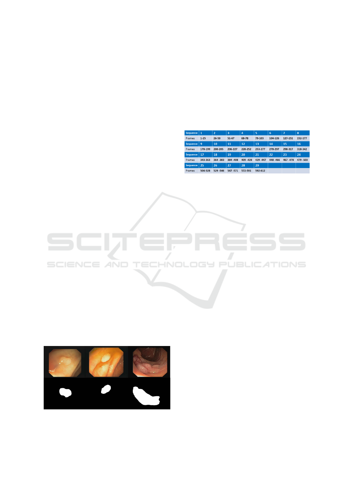
The Data-set used for the experimentation purposes is

’Polyp-CVC-CliniDB (Bernal, 2015).

Figure 3: Content of CVC-ClinicDB database.

CVC-ClinicDB is a database of frames extracted

from colonoscopy videos. These frames contain sev-

eral examples of polyps. In addition to the frames,

it consists of the ground truth for the polyps.This

ground truth consists of a mask corresponding to

the region covered by the polyp in the image.CVC-

ClinicDB database consists of two different types of

images: Original images and Polyp mask. CVC-

ClinicDB is the ofﬁcial database used in the training

stages of MICCAI 2015 Sub-Challenge on Automatic

Polyp Detection Challenge in Colonoscopy Videos.

Figure 4: Correspondence between number of frames and

video sequences in CVC-ClinicDB.

4 PROPOSED METHODS

This paper proposes two methods to classify and clus-

ter the Endoscopic polyp images. One method is us-

ing self organizing map. This method uses princi-

ples of competitive learning. Competitive learning

is a form of learning in artiﬁcial neural network in

which nodes compete for the right to respond to a sub-

set of the input data. Competitive learning works by

increasing the specialization of each node in the net-

work. In contrast to other standard Neural networks, it

only has input and output layers. There are no hidden

layers in between, instead there is a SOM layer. Train-

ing is done by competitive learning where the weights

associated with output layer nodes compete for acti-

vation. Therefore we can understand a high dimen-

sional data in less dimensions and these observations

can be classiﬁed into clusters. The second method in-

volves use of CNN. A new CNN model was generated

to classify Stain Narrow Band Endoscopic images

into Benign and Malignant classes.Images are pre-

processed using combination of Bilateral and Guided

ﬁlter which are then used as inputs to the network.

4.1 Convolutional Neural Network

A Convolutional Neural Network (CNN) is com-

prised of one or more convolutional layers (often with

a subsampling step) and then followed by one or more

fully connected layers as in a standard multilayer neu-

ral network. The architecture of a CNN is designed

to take advantage of the 2D structure of an input im-

age. This is achieved with local connections and tied

Polyp Classiﬁcation and Clustering from Endoscopic Images using Competitive and Convolutional Neural Networks

447

Figure 5: Working of SOM.

weights followed by some form of pooling which re-

sults in translation invariant features.(A. Krizhevsky

and Hinton, 2012)

Figure 6: Designed Neural Network structure.

A self designed and trained layer structure as

shown in ﬁgure 4 was used to classify Benign and

Malignant polyps. Input images were processed us-

ing smoothing ﬁlters and edges were detected. This

network was trained using 500 images of both kinds.

K-fold cross validation (Burman, 1989) was used on

this set. k-fold cross validation is a procedure used to

estimate the skill of the model on new data. In this

case we used 10-fold cross validation.

Figure 7: 10-fold cross validation.

In k-fold cross-validation, the original sample is

randomly partitioned into k equal sized subsamples.

Of the k subsamples, a single subsample is retained

as the validation data for testing the model, and the

remaining subsamples are used as training data. The

cross-validation process is then repeated k times, with

each of the k subsamples used exactly once as the val-

idation data. The k results can then be averaged to

produce a single estimation. The advantage of this

method over repeated random sub-sampling is that all

observations are used for both training and validation,

and each observation is used for validation exactly

once.

Results when compared with other pre-existing

networks were found to be less accurate than this net-

work. Accuracy of around 91 percent was achieved

while no other model could give accuracy of more

than 90 percent.

Table 1: Accuracy using different network architectures.

Network Architecture Accuracy

Lenet 82.7%

VGG 16 79.3%

VGG 19 87.8 %

Proposed Architecture 90.8%

Figure 8: Results using CNN.

4.2 Self Organizing Map

The SOM algorithm (Kohonen, 2013) is based on

competitive learning. It provides a topology preserv-

ing mapping from the high dimensional space to neu-

rons. Our brain is subdivided into specialized areas,

they speciﬁcally respond to certain stimuli i.e. stim-

uli of the same kind activate a particular region of the

brain. The idea is transposed to a competitive learning

system where the input space is ”mapped” in a small

(often rectangular) space with the following princi-

ple: similar individuals in the initial space will be pro-

jected into the same neuron or, at least, in neighboring

neurons in the output space (preservation of proxim-

ity). Neurons usually form a two-dimensional lattice

and forms a mapping from high dimensional space

onto a 2-dimensional plane in our case.Topology pre-

serving property means that the mapping preserves

the relative distance between the points. Points that

ICPRAM 2019 - 8th International Conference on Pattern Recognition Applications and Methods

448

are near each other in the input space are mapped

to nearby map units in the SOM. The SOM can thus

serve as a cluster analyzing tool of high-dimensional

data. Also, the SOM has the capability to generalize.

Generalization capability means that the network can

recognize or characterize inputs it has never encoun-

tered before.

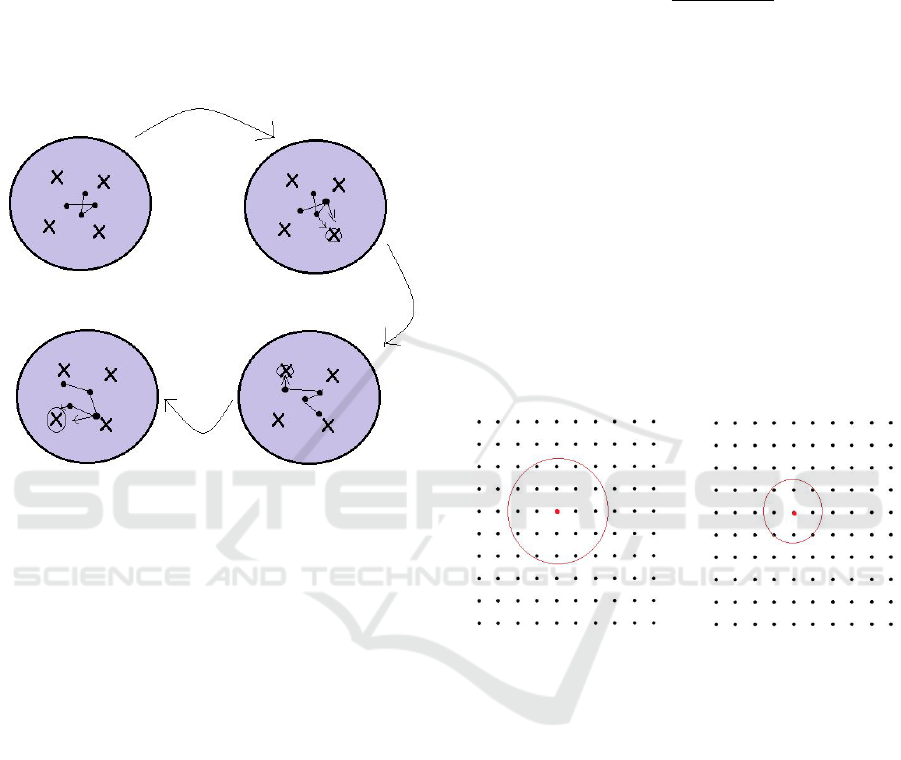
4.2.1 Learning Algorithm

Figure 9: Forming of Map.

These following steps are implemented so that the

weight vectors can represent the input data.

Step I: Randomly initialize the weights.

Step II: From the Input data, randomly choose a

point (marked in circle).

Step III: Find the weight vector which is closest

to the point chosen in previous step. This is consid-

ered as the winning neuron.

Step IV: The winning neuron and it’s closest

neighbouring neuron move closer to this chosen

point. Neurons which are closer to this point are

supposed to take larger steps than their neighbouring

neurons.

Step V: These steps are repeated many times

and it results in the weight vectors to settle into stable

zones that represent the patterns in the input data.

The step size for updating the weights and the

amount of weights to be updated decreases across

iterations

For ﬁnding the Best matching unit, we iterate

through all the nodes and compare the Euclidean dis-

tance between every node’s weight vector and present

input vector. Node with weight vector closest to in-

put vector is termed as the best matching unit for that

particular input. This Euclidean distance can be cal-

culated using:

dist =

∑

i=0

−W

)

where V is current input vector and W is node’s

weight vector.

Once this best matching unit is decided, we ﬁnd all the

other node’s which are in it’s neighbourhood because

in next step all their weights will be altered. Number

of node’s coming in a BMU’s neighbourhood depends

on the radius of neighbourhood chosen. This area of

neighbourhood will keep on shrinking with every iter-

ation. This property is visualized by the exponential

decay function.

σ(t) = σ

−t/λ

where σ

denotes the width of the lattice at time t=0,

λ denotes the time constant and t represents current

iteration of the loop.

Figure 10: Shrinking of radius.

This radius will keep shrinking until only one neu-

ron that is the BMU is present inside the neighbour-

hood. Weight vector of every node present inside the

current neighbourhood is updated using

W (t + 1) = W (t) + θ(t)L(t)(V (t)−W(t))

where t is the time step, L is the learning rate which

decays with time using

L(t) = L

−t/λ

Now practical use suggests that not only the Learn-

ing rate should decay with iteration but also it’s effect

should decrease as the distance from the best match-

ing unit increase. There should barely be any effect

at edges of the neighbourhood. To fade the amount

of learning with increasing distance Gaussian decay

function is used. θ deﬁnes the amount of inﬂuence on

learning rate of a node with distance ’dist’ from BMU

will have.

θ(t) = e

−dist

/2σ(t)

)

Polyp Classiﬁcation and Clustering from Endoscopic Images using Competitive and Convolutional Neural Networks

449

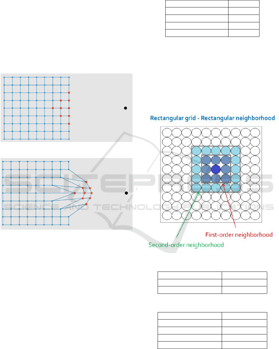
Neuron grid that is used is 2 dimensional rectangular

grid. Therefore each neuron is connected directly to 4

other neurons which are it’s close neighbours. Every

neuron possess two properties that is connection to

other neurons and position. Connections are deﬁned

before the start of training and that remain same in all

the iterations whereas the positions keep on changing.

Positions of these neurons were initialized randomly.

At the end of every iteration the position of the win-

ning neuron and all the neurons in it’s neighbourhood

are updated.

Figure 11: Feature map before training.

Figure 12: Feature map after training.

5 RESULTS

5.1 Using CNN

Around 500 images of Benign and Malignant Polyps

were used as input to Neural networks after neces-

sary pre-processing. Different kinds of architectures

of neural networks were used to compare the results.

K-fold Cross Validation was used on this set. k-

fold cross validation is a procedure used to estimate

the skill of the model on new data. In this case we

used 10-fold cross validation. Accuracy achieved us-

ing these networks is shown in Table 1. Maximum

accuracy was achieved using the proposed Network

structure while minimum accuracy was achieved us-

ing VGG16.

Table 2: Accuracy using different network architectures.

Network Architecture Accuracy

Lenet 82.7%

VGG 16 79.3%

VGG 19 87.8 %

Proposed Architecture 90.8%

5.2 Clustering

5.2.1 Implementation

The grid structure proposed in our method is Rectan-

gular grid - Rectangular neighbourhood. The notion

of neighborhood is essential in SOM, especially for

the updating of weights and their propagation during

the learning process.

Figure 13: Rectangular grid.

Table 3: Image data statistics for 2 class clustering.

Image Type No. of samples

White Light Benign 104

White Light Malignant 92

Table 4: Image data statistics for 4 class clustering.

Image Type No. of samples

White Light Benign 60

White Light Malignant 60

Stain NBI Benign 60

Stain NBI Malignant 60

The further the neighbouring neuron is from win-

ning neuron, smaller it’s learning rate will be and

smaller the std parameter, smaller will be learning rate

for neighbouring neurons.

ICPRAM 2019 - 8th International Conference on Pattern Recognition Applications and Methods

450

Parameters used for the Competitive Neural network:

i) Initial Learning Radius: 6

ii) Reduce radius after: 5 Epochs

iii) std = 1

iv) reduce std after: 5 Epochs

v) step= 0.1

vi) Reduce step after: 5 Epochs

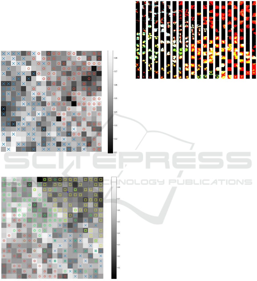
5.2.2 Formation of Clusters

Figure 14: Clustering of White Light Benign and Malignant

polyp.

Figure 15: Clustering of White Light Benign, Malig-

nant,Stain NBI Benign , Malignant Polyp.

Where square represents StainNBI Benign, pentagon

is StainNBI Malignant, cross represent White Light

Benign and Circle shows White Light Malignant.

Each Cell in this heatmap has a number associ-

ated with it which represents it’s average distance to

neighbour clusters. This number can be interpreted

from the color bar. White color means that this clus-

ter is far from it’s neighbours.

Figure 16: 4-class original cluster.

Figure 10 and 11 shows the formation of clusters

according to the similarity in the structure of in-

put polyps. Different symbols are used to represent

polyps belonging to different classes. Polyp struc-

tures which are predicted to be of similar shapes tend

to remain closer than those with different shapes. Fig-

ure 12 contains original images from the reduced data

set. This ﬁgure can be used to carefully understand

the relation between a new polyp data with those

which occurred in past.

6 CONCLUSION

Thus the CNN Architecture proposed in this paper

can be used for efﬁcient classiﬁcation of Benign and

Malignant Polyps from the Endoscopic scene. Such

kind of automatic classiﬁcation can lead to easy di-

agnosis of tumor at early stage and further course of

treatment can be decided effectively. Figure 12 shown

above can be further used for real time treatment pre-

diction if proper data is provided.

Further development in this approach can be made

so that a doctor can see similar past cases and makes

a judgment depending on the outcomes of previous

decision thus decreasing the chances of fatality. The

kind of treatment given in previous cases can also be

provided as input to facilitate automatic prediction of

course of treatment using the information on how the

actual doctor proceeded in the previous cases of sim-

ilar polyp structure

Polyp Classiﬁcation and Clustering from Endoscopic Images using Competitive and Convolutional Neural Networks

451

ACKNOWLEDGMENT

Iwahori’s research is supported by JSPS Grant-in-Aid

for Scientiﬁc Research (C) (17K00252) and Chubu

University Grant.

REFERENCES

A. Krizhevsky, I. S. and Hinton, G. E. (2012). Ima-

genet classiﬁcation with deep convolutional neural

networks,. Advances in neural information pro- cess-

ing systems.

A. Sharif Razavian, H. Azizpour, J. S. and Carlsson, S.

(2014). Cnn features off-the-shelf: an astounding

baseline for recognition. Proceedings of the IEEE

Conference on Computer Vision and Pattern Recog-

nition Workshops.

Ahmed, N. (2015). Recent review on image clustering. IET

Image Processing.

Bernal, J., S. F. J. F.-E. G. G. D. R. C. . V. F. (2015).

Wm-dova maps for accurate polyp highlighting in

colonoscopy: Validation vs. saliency maps from

physicians. computerized medical imaging and graph-

ics.

Burman, P. (1989). A comparative study of ordinary cross-

validation, v-fold cross-validation and the repeated

learning-testing methods.

Coleman, G. B. and Andrews, H. C. (1979). Image segmen-

tation by clustering. Proceedings of the IEEE.

J. Bernal, F. J. Sanchez, F. E. G. and Rodriguez, C. Cvc

clinicdb.

Kohonen, T. (2013). Essentials of the self-organizing map.

Neural networks : the ofﬁcial journal of the Interna-

tional Neural Network Society.

Nath, S. S., Mishra, G., Kar, J., Chakraborty, S., and Dey,

N. (2014). A survey of image classiﬁcation methods

and techniques. In 2014 International Conference on

Control, Instrumentation, Communication and Com-

putational Technologies (ICCICCT).

Simonyan, K. and Zisserman, A. (2014). Very deep con-

volutional networks for large-scale image recognition.

arXiv preprint arXiv:1409. 1556.

Tajbakhsh, N. (2016). Convolutional neural networks for

medical image analysis: Full training or ﬁne tuning?

In IEEE Transactions on Medical Imaging.

Y.Iwahori, T.Shinohara, A. R. S. M. and K.Kasugai (2013).

Automatic polyp detection in endoscope images using

a hessian ﬁlter. In MVA.

Zhao, Z. and Ma, Q. (2014). A novel method for image

clustering. In 2014 10th International Conference on

Natural Computation (ICNC).

ICPRAM 2019 - 8th International Conference on Pattern Recognition Applications and Methods

452