Improving Unsupervised Defect Segmentation

by Applying Structural Similarity to Autoencoders

Paul Bergmann

, Sindy L

owe

1,2

, Michael Fauser

, David Sattlegger

and Carsten Steger

MVTec Software GmbH, Germany

University of Amsterdam, The Netherlands

Keywords:

Unsupervised Learning, Anomaly Detection, Defect Segmentation.

Abstract:

Convolutional autoencoders have emerged as popular methods for unsupervised defect segmentation on image

data. Most commonly, this task is performed by thresholding a per-pixel reconstruction error based on an

-distance. This procedure, however, leads to large residuals whenever the reconstruction includes slight

localization inaccuracies around edges. It also fails to reveal defective regions that have been visually altered

when intensity values stay roughly consistent. We show that these problems prevent these approaches from

being applied to complex real-world scenarios and that they cannot be easily avoided by employing more

elaborate architectures such as variational or feature matching autoencoders. We propose to use a perceptual

loss function based on structural similarity that examines inter-dependencies between local image regions,

taking into account luminance, contrast, and structural information, instead of simply comparing single pixel

values. It achieves signiﬁcant performance gains on a challenging real-world dataset of nanoﬁbrous materials

and a novel dataset of two woven fabrics over state-of-the-art approaches for unsupervised defect segmentation

that use per-pixel reconstruction error metrics.

1 INTRODUCTION

Visual inspection is essential in industrial manufac-

turing to ensure high production quality and high

cost efﬁciency by quickly discarding defective parts.

Since manual inspection by humans is slow, expen-

sive, and error-prone, the use of fully automated com-

puter vision systems is becoming increasingly popu-

lar. Supervised methods, where the system learns

how to segment defective regions by training on both

defective and non-defective samples, are commonly

used. However, they involve a large effort to annotate

data and all possible defect types need to be known

beforehand. Furthermore, in some production pro-

cesses, the scrap rate might be too small to produce

a sufﬁcient number of defective samples for training,

especially for data-hungry deep learning models.

In this work, we focus on unsupervised defect seg-

mentation for visual inspection. The goal is to seg-

ment defective regions in images after having trai-

ned exclusively on non-defective samples. It has been

shown that architectures based on convolutional neu-

ral networks (CNNs) such as autoencoders (Goodfel-

low et al., 2016) or generative adversarial networks

(GANs) (Goodfellow et al., 2014) can be used for this

task. We provide a brief overview of such methods in

Section 2. These models try to reconstruct their in-

puts in the presence of certain constraints such as a

bottleneck and thereby manage to capture the essence

of high-dimensional data (e.g., images) in a lower-

dimensional space. It is assumed that anomalies in

the test data deviate from the training data manifold

and the model is unable to reproduce them. As a re-

sult, large reconstruction errors indicate defects. Ty-

pically, the error measure that is employed is a per-

pixel `

-distance, which is an ad-hoc choice made for

the sake of simplicity and speed. However, these me-

asures yield high residuals in locations where the re-

construction is only slightly inaccurate, e.g., due to

small localization imprecisions of edges. They also

fail to detect structural differences between the input

and reconstructed images when the respective pixels’

color values are roughly consistent. We show that this

limits the usefulness of such methods when employed

in complex real-world scenarios.

To alleviate the aforementioned problems, we

propose to measure reconstruction accuracy using

the structural similarity (SSIM) metric (Wang et al.,

2004). SSIM is a distance measure designed to cap-

ture perceptual similarity that is less sensitive to edge

372

Bergmann, P., Löwe, S., Fauser, M., Sattlegger, D. and Steger, C.

Improving Unsupervised Defect Segmentation by Applying Structural Similarity to Autoencoders.

DOI: 10.5220/0007364503720380

In Proceedings of the 14th International Joint Conference on Computer Vision, Imaging and Computer Graphics Theory and Applications (VISIGRAPP 2019), pages 372-380

ISBN: 978-989-758-354-4

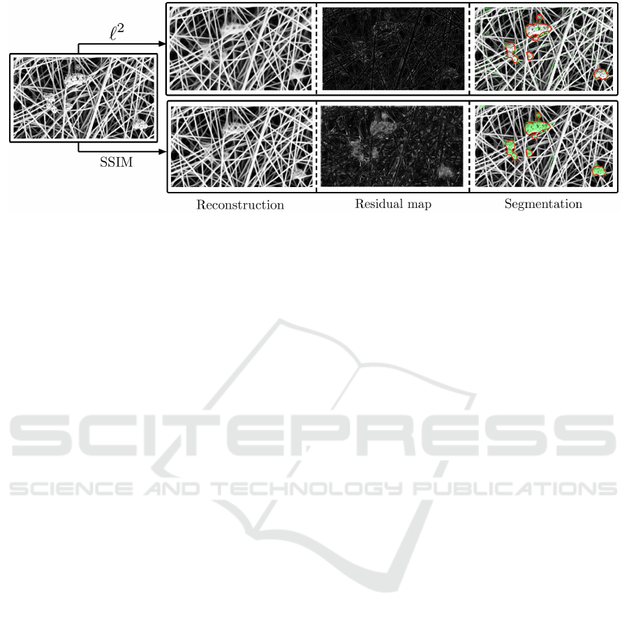
Figure 1: A defective image of nanoﬁbrous materials is reconstructed by an autoencoder optimizing either the commonly

used pixel-wise `

-distance or a perceptual similarity metric based on structural similiarity (SSIM). Even though an `

autoencoder fails to properly reconstruct the defects, a per-pixel comparison of the original input and reconstruction does not

yield signiﬁcant residuals that would allow for defect segmentation. The residual map using SSIM puts more importance on

the visually salient changes made by the autoencoder, enabling for an accurate segmentation of the defects.

alignment and gives importance to salient differences

between input and reconstruction. It captures inter-

dependencies between local pixel regions that are dis-

regarded by the current state-of-the-art unsupervised

defect segmentation methods based on autoencoders

with per-pixel losses. We evaluate the performance

gains obtained by employing SSIM as a loss function

on two real-world industrial inspection datasets and

demonstrate signiﬁcant performance gains over per-

pixel approaches. Figure 1 demonstrates the advan-

tage of perceptual loss functions over a per-pixel `

loss on the NanoTWICE dataset of nanoﬁbrous ma-

terials (Carrera et al., 2017). While both autoen-

coders alter the reconstruction in defective regions,

only the residual map of the SSIM autoencoder al-

lows a segmentation of these areas. By changing the

loss function and otherwise keeping the same autoen-

coding architecture, we reach a performance that is

on par with other state-of-the-art unsupervised defect

segmentation approaches that rely on additional mo-

del priors such as handcrafted features or pretrained

networks.

2 RELATED WORK

Detecting anomalies that deviate from the training

data has been a long-standing problem in machine le-

arning. Pimentel et al. (Pimentel et al., 2014) give

a comprehensive overview of the ﬁeld. In compu-

ter vision, one needs to distinguish between two va-

riants of this task. First, there is the classiﬁcation sce-

nario, where novel samples appear as entirely diffe-

rent object classes that should be predicted as out-

liers. Second, there is a scenario where anomalies

manifest themselves in subtle deviations from other-

wise known structures and a segmentation of these

deviations is desired. For the classiﬁcation problem,

a number of approaches have been proposed (Perera

and Patel, 2018; Sabokrou et al., 2018). Here, we li-

mit ourselves to an overview of methods that attempt

to tackle the latter problem.

(Napoletano et al., 2018) extract features from a

CNN that has been pretrained on a classiﬁcation task.

The features are clustered in a dictionary during trai-

ning and anomalous structures are identiﬁed when the

extracted features strongly deviate from the learned

cluster centers. General applicability of this appro-

ach is not guaranteed since the pretrained network

might not extract useful features for the new task at

hand and it is unclear which features of the network

should be selected for clustering. The results achieved

with this method are the current state-of-the-art on the

NanoTWICE dataset, which we also use in our expe-

riments. They improve upon previous results by (Car-

rera et al., 2017), who build a dictionary that yields a

sparse representation of the normal data. Similar ap-

proaches using sparse representations for novelty de-

tection are (Boracchi et al., 2014; Carrera et al., 2015;

Carrera et al., 2016).

(Schlegl et al., 2017) train a GAN on optical cohe-

rence tomography images of the retina and detect ano-

malies such as retinal ﬂuid by searching for a latent

sample that minimizes the per-pixel `

-reconstruction

error as well as a discriminator loss. The large number

of optimization steps that must be performed to ﬁnd a

suitable latent sample makes this approach very slow.

Therefore, it is only useful in applications that are not

time-critical. Recently, (Zenati et al., 2018) proposed

to use bidirectional GANs (Donahue et al., 2017) to

add the missing encoder network for faster inference.

Improving Unsupervised Defect Segmentation by Applying Structural Similarity to Autoencoders

373

However, GANs are prone to run into mode collapse,

i.e., there is no guarantee that all modes of the dis-

tribution of non-defective images are captured by the

model. Furthermore, they are more difﬁcult to train

than autoencoders since the loss function of the ad-

versarial training typically cannot be trained to con-

vergence (Arjovsky and Bottou, 2017). Instead, the

training results must be judged manually after regular

optimization intervals.

(Baur et al., 2018) propose a framework for defect

segmentation using autoencoding architectures and a

per-pixel error metric based on the `

-distance. To

prevent the disadvantages of their loss function, they

improve the reconstruction quality by requiring alig-

ned input data and adding an adversarial loss to en-

hance the visual quality of the reconstructed images.

However, for many applications that work on unstruc-

tured data, prior alignment is impossible. Further-

more, optimizing for an additional adversarial loss

during training but simply segmenting defects ba-

sed on per-pixel comparisons during evaluation might

lead to worse results since it is unclear how the adver-

sarial training inﬂuences the reconstruction.

Other approaches take into account the structure

of the latent space of variational autoencoders (VAEs)

(Kingma and Welling, 2014) in order to deﬁne mea-

sures for outlier detection. (An and Cho, 2015) de-

ﬁne a reconstruction probability for every image pixel

by drawing multiple samples from the estimated en-

coding distribution and measuring the variability of

the decoded outputs. (Soukup and Pinetz, 2018) dis-

regard the decoder output entirely and instead com-

pute the KL divergence as a novelty measure between

the prior and the encoder distribution. This is ba-

sed on the assumption that defective inputs will mani-

fest themselves in mean and variance values that are

very different from those of the prior. Similarly, (Va-

silev et al., 2018) deﬁne multiple novelty measures,

either by purely considering latent space behavior or

by combining these measures with per-pixel recon-

struction losses. They obtain a single scalar value

that indicates an anomaly, which can quickly become

a performance bottleneck in a segmentation scenario

where a separate forward pass would be required for

each image pixel to obtain an accurate segmentation

result. We show that per-pixel reconstruction proba-

bilities obtained from VAEs suffer from the same pro-

blems as per-pixel deterministic losses (cf. Section 4).

All the aforementioned works that use autoen-

coders for unsupervised defect segmentation have

shown that autoencoders reliably reconstruct non-

defective images while visually altering defective re-

gions to keep the reconstruction close to the learned

manifold of the training data. However, they rely on

per-pixel loss functions that make the unrealistic as-

sumption that neighboring pixel values are mutually

independent. We show that this prevents these appro-

aches from segmenting anomalies that differ predomi-

nantly in structure rather than pixel intensity. Instead,

we propose to use SSIM (Wang et al., 2004) as the

loss function and measure of anomaly by comparing

input and reconstruction. SSIM takes interdependen-

cies of local patch regions into account and evaluates

their ﬁrst and second order moments to model diffe-

rences in luminance, contrast, and structure. (Rid-

geway et al., 2015) show that SSIM and the closely

related multi-scale version MS-SSIM (Wang et al.,

2003) can be used as differentiable loss functions to

generate more realistic images in deep architectures

for tasks such as superresolution, but do not examine

its usefulness for defect segmentation in an autoen-

coding framework. In all our experiments, switching

from per-pixel to perceptual losses yields signiﬁcant

gains in performance, sometimes enhancing the met-

hod from a complete failure to a satisfactory defect

segmentation result.

3 METHODOLOGY

3.1 Autoencoders for Unsupervised

Defect Segmentation

Autoencoders attempt to reconstruct an input image

x ∈ R

k×h×w

through a bottleneck, effectively pro-

jecting the input image into a lower-dimensional

space, called latent space. An autoencoder consists

of an encoder function E : R

k×h×w

→ R

and a deco-

der function D : R

→ R

k×h×w

, where d denotes the

dimensionality of the latent space and k, h,w denote

the number of channels, height, and width of the in-

put image, respectively. Choosing d  k ×h × w pre-

vents the architecture from simply copying its input

and forces the encoder to extract meaningful features

from the input patches that facilitate accurate recon-

struction by the decoder. The overall process can be

summarized as

x = D(E(x)) = D(z) , (1)

where z is the latent vector and

x the reconstruction

of the input. In our experiments, the functions E and

D are parameterized by CNNs. Strided convolutions

are used to down-sample the input feature maps in the

encoder and to up-sample them in the decoder. Au-

toencoders can be employed for unsupervised defect

segmentation by training them purely on defect-free

image data. During testing, the autoencoder will fail

VISAPP 2019 - 14th International Conference on Computer Vision Theory and Applications

374

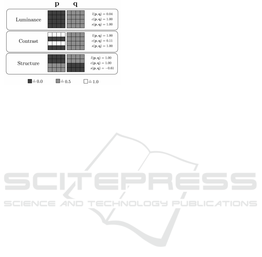
Figure 2: Different responsibilities of the three similarity

functions employed by SSIM. Example patches p and q

differ in either luminance, contrast, or structure. SSIM

is able to distinguish between these three cases, assigning

close to minimum similarity values to one of the compari-

son functions l(p, q), c(p, q), or s(p,q), respectively. An

-comparison of these patches would yield a constant per-

pixel residual value of 0.25 for each of the three cases.

to reconstruct defects that have not been observed du-

ring training, which can thus be segmented by compa-

ring the original input to the reconstruction and com-

puting a residual map R(x,

x) ∈ R

w×h

3.1.1 `

-Autoencoder

To force the autoencoder to reconstruct its input,

a loss function must be deﬁned that guides it to-

wards this behavior. For simplicity and computational

speed, one often chooses a per-pixel error measure,

such as the L

loss

(x,

x) =

h−1

∑

r=0

w−1

∑

c=0

(x(r, c) −

x(r, c))

, (2)

where x(r, c) denotes the intensity value of image x

at the pixel (r, c). To obtain a residual map R

(x,

during evaluation, the per-pixel `

-distance of x and

is computed.

3.1.2 Variational Autoencoder

Various extensions to the deterministic autoencoder

framework exist. VAEs (Kingma and Welling, 2014)

impose constraints on the latent variables to follow

a certain distribution z ∼ P(z). For simplicity, the

distribution is typically chosen to be a unit-variance

Gaussian. This turns the entire framework into a pro-

babilistic model that enables efﬁcient posterior infe-

rence and allows to generate new data from the trai-

ning manifold by sampling from the latent distribu-

tion. The approximate posterior distribution Q(z|x)

obtained by encoding an input image can be used

to deﬁne further anomaly measures. One option is

to compute a distance between the two distributi-

ons, such as the KL-divergence K L(Q(z|x)||P(z)),

and indicate defects for large deviations from the

prior P(z) (Soukup and Pinetz, 2018). However, to

use this approach for the pixel-accurate segmenta-

tion of anomalies, a separate forward pass for each

pixel of the input image would have to be perfor-

med. A second approach for utilizing the posterior

Q(z|x) that yields a spatial residual map is to decode

N latent samples z

,. . ., z

drawn from Q(z|x) and

to evaluate the per-pixel reconstruction probability

VAE

= P(x|z

,. . ., z

) as described by (An and

Cho, 2015).

3.1.3 Feature Matching Autoencoder

Another extension to standard autoencoders was pro-

posed by (Dosovitskiy and Brox, 2016). It increa-

ses the quality of the produced reconstructions by ex-

tracting features from both the input image x and its

reconstruction

x and enforcing them to be equal. Con-

sider F : R

k×h×w

→ R

to be a feature extractor that

obtains an f -dimensional feature vector from an in-

put image. Then, a regularizer can be added to the

loss function of the autoencoder, yielding the feature

matching autoencoder (FM-AE) loss

(x,

x) = L

(x,

x) + λkF(x) − F(

x)k

, (3)

where λ > 0 denotes the weighting factor between the

two loss terms. F can be parameterized using the ﬁrst

layers of a CNN pretrained on an image classiﬁcation

task. During evaluation, a residual map R

is obtai-

ned by comparing the per-pixel `

-distance of x and

The hope is that sharper, more realistic reconstructi-

ons will lead to better residual maps compared to a

standard `

-autoencoder.

3.1.4 SSIM Autoencoder

We show that employing more elaborate architectures

such as VAEs or FM-AEs does not yield satisfactory

improvements of the residial maps over deterministic

-autoencoders in the unsupervised defect segmen-

tation task. They are all based on per-pixel evalua-

tion metrics that assume an unrealistic independence

between neighboring pixels. Therefore, they fail to

detect structural differences between the inputs and

their reconstructions. By adapting the loss and eva-

luation functions to capture local inter-dependencies

between image regions, we are able to drastically im-

prove upon all the aforementioned architectures. In

Section 3.2, we speciﬁcally motivate the use of the

strucutural similarity metric SSIM(x,

x) as both the

loss function and the evaluation metric for autoenco-

ders to obtain a residual map R

SSIM

Improving Unsupervised Defect Segmentation by Applying Structural Similarity to Autoencoders

375

(a)

(b)

(c)

(d)

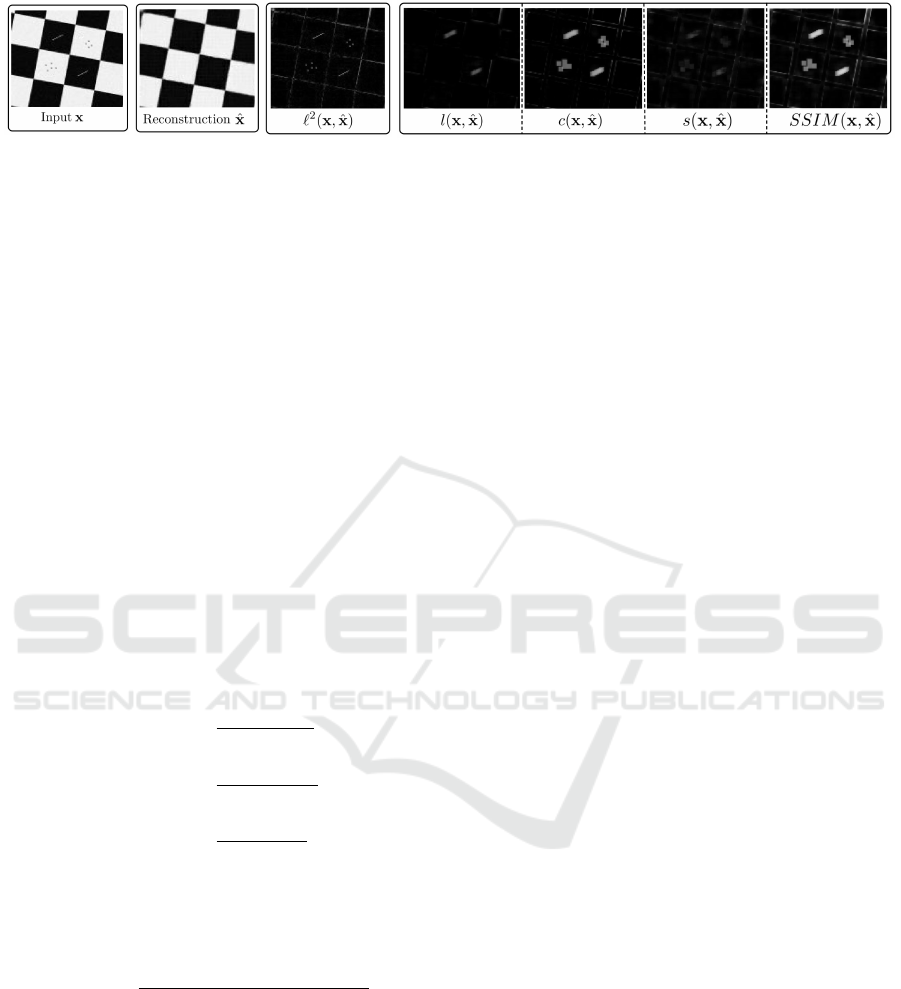
Figure 3: A toy example illustrating the advantages of SSIM over `

for the segmentation of defects. (a) 128 × 128 chec-

kerboard pattern with gray strokes and dots that simulate defects. (b) Output reconstruction

x of the input image x by an

-autoencoder trained on defect-free checkerboard patterns. The defects have been removed by the autoencoder. (c) `

residual map. Brighter colors indicate larger dissimilarity between input and reconstruction. (d) Residuals for luminance l,

contrast c, structure s, and their pointwise product that yields the ﬁnal SSIM residual map. In contrast to the `

-error map,

SSIM gives more importance to the visually more salient disturbances than to the slight inaccuracies around reconstructed

edges.

3.2 Structural Similarity

The SSIM index (Wang et al., 2004) deﬁnes a dis-

tance measure between two K × K image patches p

and q, taking into account their similarity in lumi-

nance l(p, q), contrast c(p,q), and structure s(p, q):

SSIM(p,q) = l(p, q)

c(p,q)

s(p,q)

, (4)

where α,β,γ ∈ R are user-deﬁned constants to weight

the three terms. The luminance measure l(p,q) is es-

timated by comparing the patches’ mean intensities

and µ

. The contrast measure c(p, q) is a function

of the patch variances σ

and σ

. The structure mea-

sure s(p,q) takes into account the covariance σ

the two patches. The three measures are deﬁned as:

l(p, q) =

2µ

+ c

+ µ

+ c

(5)

c(p,q) =

2σ

+ c

+ σ

+ c

(6)

s(p,q) =

2σ

+ c

2σ

+ c

. (7)

The constants c

and c

ensure numerical stability and

are typically set to c

= 0.01 and c

= 0.03. By sub-

stituting (5)-(7) into (4), the SSIM is given by

SSIM(p,q) =

(2µ

+ c

)(2σ

+ c

)

(µ

+ µ

+ c

)(σ

+ σ

+ c

)

. (8)

It holds that SSIM(p, q) ∈ [−1,1]. In particular,

SSIM(p,q) = 1 if and only if p and q are identi-

cal (Wang et al., 2004). Figure 2 shows the diffe-

rent perceptions of the three similarity functions that

form the SSIM index. Each of the patch pairs p and

q has a constant `

-residual of 0.25 per pixel and

hence assigns low defect scores to each of the three

cases. SSIM on the other hand is sensitive to variati-

ons in the patches’ mean, variance, and covariance in

its respective residual map and assigns low similarity

to each of the patch pairs in one of the comparison

functions.

To compute the structural similarity between an

entire image x and its reconstruction

x, one slides a

K ×K window across the image and computes a SSIM

value at each pixel location. Since (8) is differentia-

ble, it can be employed as a loss function in deep le-

arning architectures that are optimized using gradient

descent.

Figure 3 indicates the advantages SSIM has over

per-pixel error functions such as `

for segmenting de-

fects. After training an `

-autoencoder on defect-free

checkerboard patterns of various scales and orien-

tations, we apply it to an image (Figure 3(a)) that

contains gray strokes and dots that simulate defects.

Figure 3(b) shows the corresponding reconstruction

produced by the autoencoder, which removes the de-

fects from the input image. The two remaining subﬁ-

gures display the residual maps when evaluating the

reconstruction error with a per-pixel `

-comparison

or SSIM. For the latter, the luminance, contrast, and

structure maps are also shown. For the `

-distance,

both the defects and the inaccuracies in the recon-

struction of the edges are weighted equally in the er-

ror map, which makes them indistinguishable. Since

SSIM computes three different statistical features for

image comparison and operates on local patch regi-

ons, it is less sensitive to small localization inaccu-

racies in the reconstruction. In addition, it detects de-

fects that manifest themselves in a change of structure

rather than large differences in pixel intensity. For the

defects added in this particular toy example, the con-

trast function yields the largest residuals.

VISAPP 2019 - 14th International Conference on Computer Vision Theory and Applications

376

(a) (b)

(c)

(d)

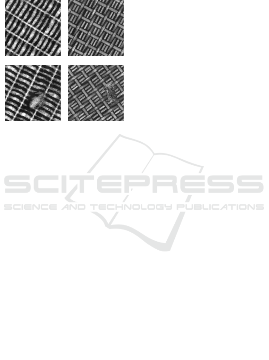
Figure 4: Example images from the contributed texture da-

taset of two woven fabrics. (a) and (b) show examples of

non-defective textures that can be used for training. (c) and

(d) show exemplary defects for both datasets. See the text

for details.

4 EXPERIMENTS

4.1 Datasets

Due to the lack of datasets for unsupervised defect

segmentation in industrial scenarios, we contribute a

novel dataset of two woven fabric textures, which is

available to the public

. We provide 100 defect-free

images per texture for training and validation and 50

images that contain various defects such as cuts, roug-

hened areas, and contaminations on the fabric. Pixel-

accurate ground truth annotations for all defects are

also provided. All images are of size 512 ×512 pixels

and were acquired as single-channel gray-scale ima-

ges. Examples of defective and defect-free textures

can be seen in Figure 4. We further evaluate our

method on a dataset of nanoﬁbrous materials (Car-

rera et al., 2017), which contains ﬁve defect-free gray-

scale images of size 1024 × 700 for training and va-

lidation and 40 defective images for evaluation. A

sample image of this dataset is shown in Figure 1.

4.2 Training and Evaluation Procedure

For all datasets, we train the autoencoders with their

respective losses and evaluation metrics, as descri-

The dataset will be made available at http://www.

mvtec.com/company/research/publications.

Table 1: General outline of our autoencoder architecture.

The depicted values correspond to the structure of the enco-

der. The decoder is built as a reversed version of this. Leaky

rectiﬁed linear units (ReLUs) with slope 0.2 are applied as

activation functions after each layer except for the output

layers of both the encoder and the decoder, in which linear

activation functions are used.

Layer Output Size Parameters

Kernel Stride Padding

Input 128x128x1

Conv1 64x64x32 4x4 2 1

Conv2 32x32x32 4x4 2 1

Conv3 32x32x32 3x3 1 1

Conv4 16x16x64 4x4 2 1

Conv5 16x16x64 3x3 1 1

Conv6 8x8x128 4x4 2 1

Conv7 8x8x64 3x3 1 1

Conv8 8x8x32 3x3 1 1

Conv9 1x1xd 8x8 1 0

bed in Section 3.1. Each architecture is trained on

10 000 defect-free patches of size 128 × 128, rand-

omly cropped from the given training images. In or-

der to capture a more global context of the textures,

we down-scaled the images to size 256 × 256 before

cropping. Each network is trained for 200 epochs

using the ADAM (Kingma and Ba, 2015) optimizer

with an initial learning rate of 2 × 10

−4

and a weight

decay set to 10

−5

. The exact parametrization of the

autoencoder network shared by all tested architectu-

res is given in Table 1. The latent space dimension

for our experiments is set to d = 100 on the texture

images and to d = 500 for the nanoﬁbres due to their

higher structural complexity. For the VAE, we decode

N = 6 latent samples from the approximate posterior

distribution Q(z|x) to evaluate the reconstruction pro-

bability for each pixel. The feature matching autoen-

coder is regularized with the ﬁrst three convolutional

layers of an AlexNet (Krizhevsky et al., 2012) pre-

trained on ImageNet (Russakovsky et al., 2015) and

a weight factor of λ = 1. For SSIM, the window size

is set to K = 11 unless mentioned otherwise and its

three residual maps are equally weighted by setting

α = β = γ = 1.

The evaluation is performed by striding over the

test images and reconstructing image patches of size

128 × 128 using the trained autoencoder and com-

puting its respective residual map R. In principle,

it would be possible to set the horizontal and verti-

cal stride to 128. However, at different spatial loca-

tions, the autoencoder produces slightly different re-

constructions of the same data, which leads to some

striding artifacts. Therefore, we decreased the stride

to 30 pixels and averaged the reconstructed pixel va-

lues. The resulting residual maps are thresholded

to obtain candidate regions where a defect might be

present. An opening with a circular structuring ele-

ment of diameter 4 is applied as a morphological post-

Improving Unsupervised Defect Segmentation by Applying Structural Similarity to Autoencoders

377

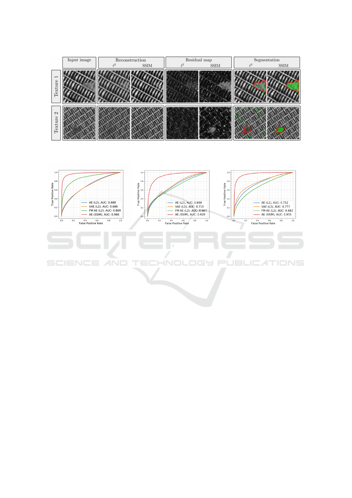
Figure 5: Qualitative comparison between reconstructions, residual maps, and segmentation results of an `

-autoencoder and

an SSIM autoencoder on two datasets of woven fabric textures. The ground truth regions containing defects are outlined in

red while green areas mark the segmentation result of the respective method.

(a)

(b) (c)

Figure 6: Resulting ROC curves of the proposed SSIM autoencoder (red line) on the evaluated datasets of nanoﬁbrous

materials (a) and the two texture datasets (b), (c) in comparison with other autoencoding architectures that use per-pixel

loss functions (green, orange, and blue lines). Corresponding AUC values are given in the legend.

processing to delete outlier regions that are only a few

pixels wide (Steger et al., 2018). We compute the re-

ceiver operating characteristic (ROC) as the evalua-

tion metric. The true positive rate is deﬁned as the

ratio of pixels correctly classiﬁed as defect across the

entire dataset. The false positive rate is the ratio of

pixels misclassiﬁed as defect.

4.3 Results

Figure 5 shows a qualitative comparison between the

performance of the `

-autoencoder and the SSIM au-

toencoder on images of the two texture datasets. Alt-

hough both architectures remove the defect in the re-

construction, only the SSIM residual map reveals the

defects and provides an accurate segmentation result.

The same can be observed for the NanoTWICE data-

set, as shown in Figure 1.

We conﬁrm this qualitative behavior by numerical

results. Figure 6 compares the ROC curves and their

respective AUC values of our approach using SSIM

to the per-pixel architectures. The performance of the

latter is often only marginally better than classifying

each pixel randomly. For the VAE, we found that

the reconstructions obtained by different latent sam-

ples from the posterior does not vary greatly. Thus,

it could not improve on the deterministic framework.

Employing feature matching only improved the seg-

mentation result for the dataset of nanoﬁbrous mate-

rials, while not yielding a beneﬁt for the two texture

datasets. Using SSIM as the loss and evaluation me-

tric outperforms all other tested architectures signi-

ﬁcantly. By merely changing the loss function, the

achieved AUC improves from 0.688 to 0.966 on the

dataset of nanoﬁbrous materials, which is compara-

ble to the state-of-the-art given in (Napoletano et al.,

2018), where values of up to 0.974 are reported. In

contrast to this method, autoencoders do not rely on

any model priors such as handcrafted features or pre-

trained networks. For the two texture datasets, similar

leaps in performance are observed.

Since the dataset of nanoﬁbrous materials contains

defects of various sizes and smaller sized defects con-

tribute less to the overall true positive rate when weig-

hting all pixel equally, we further evaluated the over-

lap of each detected anomaly region with the ground

truth for this dataset and report the p-quantiles for

p ∈ {25%, 50%, 75%} in Figure 7. For false positive

rates as low as 5%, more than 50% of the defects have

an overlap with the ground truth that is larger than

VISAPP 2019 - 14th International Conference on Computer Vision Theory and Applications

378

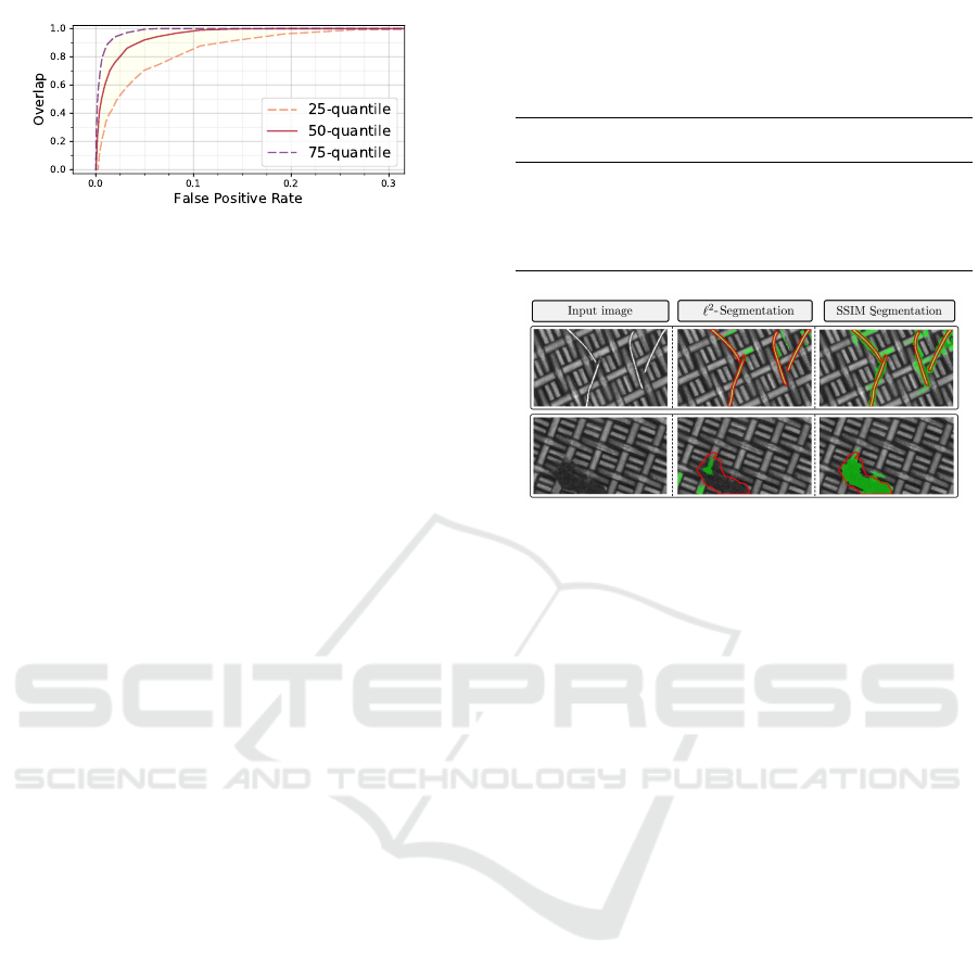
Figure 7: Per-region overlap for individual defects between

our segmentation and the ground truth for different false po-

sitive rates using an SSIM autoencoder on the dataset of na-

noﬁbrous materials.

91%. This outperforms the results achieved by (Na-

poletano et al., 2018), who report a minimal overlap

of 85% in this setting.

We further tested the sensitivity of the SSIM au-

toencoder to different hyperparameter settings. We

varied the latent space dimension d, SSIM window

size k, and the size of the patches that the autoen-

coder was trained on. Table 2 shows that SSIM is

insensitive to different hyperparameter settings once

the latent space dimension is chosen to be sufﬁciently

large. Using the optimal setup of d = 500, k = 11, and

patch size 128 × 128, a forward pass through our ar-

chitecture takes 2.23 ms on a Tesla V100 GPU. Patch-

by-patch evaluation of an entire image of the Nano-

TWICE dataset takes 3.61 s on average, which is sig-

niﬁcantly faster than the runtimes reported by (Napo-

letano et al., 2018). Their approach requires between

15 s and 55 s to process a single input image.

Figure 8 depicts qualitative advantages that em-

ploying a perceptual error metric has over per-pixel

distances such as `

. It displays two defective images

from one of the texture datasets, where the top image

contains a high-contrast defect of metal pins which

contaminate the fabric. The bottom image shows a

low-contrast structural defect where the fabric was

cut open. While the `

-norm has problems to detect

the low-constrast defect, it easily segments the metal

pins due to their large absolute distance in gray va-

lues with respect to the background. However, misa-

lignments in edge regions still lead to large residuals

in non-defective regions as well, which would make

these thin defects hard to segment in practice. SSIM

robustly segments both defect types due to its simul-

taneous focus on luminance, contrast, and structural

information and insensitivity to edge alignment due

to its patch-by-patch comparisons.

5 CONCLUSION

We demonstrate the advantage of perceptual loss

functions over commonly used per-pixel residuals in

Table 2: Area under the ROC curve (AUC) on NanoTWICE

for varying hyperparameters in the SSIM autoencoder ar-

chitecture. Different settings do not signiﬁcantly alter de-

fect segmentation performance.

Latent

dimension

AUC

SSIM

window size

AUC Patch size AUC

50 0.848 3 0.889

100 0.935 7 0.965 32 0.949

200 0.961 11 0.966 64 0.959

500 0.966 15 0.960 128 0.966

1000 0.962 19 0.952

Figure 8: In the ﬁrst row, the metal pins have a large diffe-

rence in gray values in comparison to the defect-free back-

ground material. Therefore, they can be detected by both

the `

and the SSIM error metric. The defect shown in the

second row, however, differs from the texture more in terms

of structure than in absolute gray values. As a consequence,

a per-pixel distance metric fails to segment the defect while

SSIM yields a good segmentation result.

autoencoding architectures when used for unsupervi-

sed defect segmentation tasks. Per-pixel losses fail

to capture inter-dependencies between local image

regions and therefore are of limited use when de-

fects manifest themselves in structural alterations of

the defect-free material where pixel intensity values

stay roughly consistent. We further show that em-

ploying probabilistic per-pixel error metrics obtained

by VAEs or sharpening reconstructions by feature ma-

tching regularization techniques do not improve the

segmentation result since they do not address the pro-

blems that arise from treating pixels as mutually inde-

pendent.

SSIM, on the other hand, is less sensitive to small

inaccuracies of edge locations due to its comparison

of local patch regions and takes into account three dif-

ferent statistical measures: luminance, contrast, and

structure. We demonstrate that switching from per-

pixel loss functions to an error metric based on struc-

tural similarity yields signiﬁcant improvements by

evaluating on a challenging real-world dataset of na-

noﬁbrous materials and a contributed dataset of two

woven fabric materials which we make publicly avai-

lable. Employing SSIM often achieves an enhance-

ment from almost unusable segmentations to results

that are on par with other state of the art approaches

for unsupervised defect segmentation which additi-

Improving Unsupervised Defect Segmentation by Applying Structural Similarity to Autoencoders

379

onally rely on image priors such as pre-trained net-

works.

REFERENCES

An, J. and Cho, S. (2015). Variational Autoencoder based

Anomaly Detection using Reconstruction Probability.

SNU Data Mining Center, Tech. Rep.

Arjovsky, M. and Bottou, L. (2017). Towards Principled

Methods for Training Generative Adversarial Net-

works. International Conference on Learning Repre-

sentations.

Baur, C., Wiestler, B., Albarqouni, S., and Navab, N.

(2018). Deep Autoencoding Models for Unsupervised

Anomaly Segmentation in Brain MR Images. arXiv

preprint arXiv:1804.04488.

Boracchi, G., Carrera, D., and Wohlberg, B. (2014). No-

velty Detection in Images by Sparse Representations.

In 2014 IEEE Symposium on Intelligent Embedded Sy-

stems (IES), pages 47–54. IEEE.

Carrera, D., Boracchi, G., Foi, A., and Wohlberg, B.

(2015). Detecting anomalous structures by convo-

lutional sparse models. In 2015 International Joint

Conference on Neural Networks (IJCNN), pages 1–8.

IEEE.

Carrera, D., Boracchi, G., Foi, A., and Wohlberg, B.

(2016). Scale-invariant anomaly detection with mul-

tiscale group-sparse models. In 2016 IEEE Interna-

tional Conference on Image Processing (ICIP), pages

3892–3896. IEEE.

Carrera, D., Manganini, F., Boracchi, G., and Lanzarone,

E. (2017). Defect Detection in SEM Images of Na-

noﬁbrous Materials. IEEE Transactions on Industrial

Informatics, 13(2):551–561.

Donahue, J., Kr

ahenb

uhl, P., and Darrell, T. (2017). Adver-

sarial Feature Learning. International Conference on

Learning Representations.

Dosovitskiy, A. and Brox, T. (2016). Generating Ima-

ges with Perceptual Similarity Metrics based on Deep

Networks. In Advances in Neural Information Proces-

sing Systems, pages 658–666.

Goodfellow, I., Bengio, Y., and Courville, A. (2016). Deep

Learning. MIT Press.

Goodfellow, I., Pouget-Abadie, J., Mirza, M., Xu, B.,

Warde-Farley, D., Ozair, S., Courville, A., and Ben-

gio, Y. (2014). Generative Adversarial Nets. In Ad-

vances in Neural Information Processing Systems, pa-

ges 2672–2680.

Kingma, D. P. and Ba, J. (2015). Adam: A Method for

Stochastic Optimization. International Conference on

Learning Representations.

Kingma, D. P. and Welling, M. (2014). Auto-Encoding Va-

riational Bayes. International Conference on Lear-

ning Representations.

Krizhevsky, A., Sutskever, I., and Hinton, G. E. (2012).

ImageNet Classiﬁcation With Deep Convolutional

Neural Networks. In Advances in Neural Information

Processing Systems, pages 1097–1105.

Napoletano, P., Piccoli, F., and Schettini, R. (2018). Ano-

maly Detection in Nanoﬁbrous Materials by CNN-

Based Self-Similarity. Sensors, 18(1):209.

Perera, P. and Patel, V. M. (2018). Learning Deep Fe-

atures for One-Class Classiﬁcation. arXiv preprint

arXiv:1801.05365.

Pimentel, M. A., Clifton, D. A., Clifton, L., and Tarassenko,

L. (2014). A review of novelty detection. Signal Pro-

cessing, 99:215–249.

Ridgeway, K., Snell, J., Roads, B., Zemel, R. S., and

Mozer, M. C. (2015). Learning to generate ima-

ges with perceptual similarity metrics. arXiv preprint

arXiv:1511.06409.

Russakovsky, O., Deng, J., Su, H., Krause, J., Satheesh, S.,

Ma, S., Huang, Z., Karpathy, A., Khosla, A., Bern-

stein, M., et al. (2015). ImageNet Large Scale Vi-

sual Recognition Challenge. International Journal of

Computer Vision, 115(3):211–252.

Sabokrou, M., Khalooei, M., Fathy, M., and Adeli, E.

(2018). Adversarially Learned One-Class Classiﬁer

for Novelty Detection. In Proceedings of the IEEE

Conference on Computer Vision and Pattern Recogni-

tion, pages 3379–3388.

Schlegl, T., Seeb

ock, P., Waldstein, S. M., Schmidt-Erfurth,

U., and Langs, G. (2017). Unsupervised Anomaly

Detection with Generative Adversarial Networks to

Guide Marker Discovery. In International Conference

on Information Processing in Medical Imaging, pages

146–157. Springer.

Soukup, D. and Pinetz, T. (2018). Reliably Decoding

Autoencoders’ Latent Spaces for One-Class Learning

Image Inspection Scenarios. In OAGM Workshop

2018. Verlag der Technischen Universit

at Graz.

Steger, C., Ulrich, M., and Wiedemann, C. (2018). Ma-

chine Vision Algorithms and Applications. Wiley-

VCH, Weinheim, 2nd edition.

Vasilev, A., Golkov, V., Lipp, I., Sgarlata, E., Tomassini, V.,

Jones, D. K., and Cremers, D. (2018). q-Space No-

velty Detection with Variational Autoencoders. arXiv

preprint arXiv:1806.02997.

Wang, Z., Bovik, A. C., Sheikh, H. R., and Simoncelli, E. P.

(2004). Image quality assessment: from error visi-

bility to structural similarity. IEEE transactions on

image processing, 13(4):600–612.

Wang, Z., Simoncelli, E. P., and Bovik, A. C. (2003). Mul-

tiscale structural similarity for image quality asses-

sment. In Record of the Thirty-Seventh Asilomar Con-

ference on Signals, Systems and Computers, volume 2,

pages 1398–1402. Ieee.

Zenati, H., Foo, C. S., Lecouat, B., Manek, G.,

and Chandrasekhar, V. R. (2018). Efﬁcient

GAN-Based Anomaly Detection. arXiv preprint

arXiv:1802.06222.

VISAPP 2019 - 14th International Conference on Computer Vision Theory and Applications

380