Grapheme Approach to Recognizing Letters based on Medial

Representation

Anna Lipkina and Leonid Mestetskiy

Faculty of Computational Mathematics and Cybernetics, Lomonosov Moscow State University,

Leninskiye Gory 1-52, Moscow, Russia

Keywords:

Digital Text Image, Digital Font, Grapheme, Medial Representation, Aggregated Skeleton Graph.

Abstract:

In this paper we propose a new concept of mathematical model of characters’ grapheme which nowadays is

not strictly formalized and a method of constructing graphemes based on the continuous medial representation

of letters in digital images. We also suggest the recognition method of the printed text image on the basis

of mathematical model of the grapheme used at generation of features and for classiﬁer construction. The

results of experiments conﬁrming the efﬁciency of the grapheme approach, high quality of text recognition in

different font variants and in different qualities of the text image are presented.

1 MOTIVATION

The concept of grapheme (Osetrova, 2006) is funda-

mental in writing and in reading. A literate person

recognizes letters written or printed in different fonts,

on paper or stone, on walls and on clothing. The ba-

sis of recognition is the schematic images of letters,

which are called graphemes. The grapheme is the

most general scheme of the alphabet symbol, and any

literate person, even a child, can draw it. The school

teaches reading and writing based on graphemes. Ho-

wever, text recognition software does not use this con-

cept explicitly. Graphemes are used by philologists

in their theoretical constructions, as well as designers

when creating computer fonts. Both those and others

do without the strict deﬁnition of the concept of grap-

heme. If you try to create algorithms for recognizing

the characters of the alphabet based on graphemes,

then you need to more strictly deﬁne this concept and

the ways of its description and construction.

In this article we make such an attempt. We want

to deﬁne the schematic descriptions of the characters

of the alphabet so that they can be obtained from any

font, and so that the letters can be recognized in all ot-

her fonts. To solve this problem, we propose a method

of obtaining graphemes in the form of graphs from

digital images of letters of a font and a method of re-

cognizing characters of other fonts based on a compa-

rison with graphemes. The main hypothesis is that to

build a universal set of graphemes a single type font

is enough, and the remaining fonts can be recognized

by this set. Thus, the purpose of the study is to imple-

ment and test the grapheme approach for recognizing

letters.

2 INTRODUCTION

When a literate person reads the text, he can immedi-

ately determine by the form of the symbol what let-

ter this symbol depicts. He can do it regardless of

the different variants of the artistic style of the sym-

bol (with serif, italic, straight, decorative, etc. (Para-

Type, 2008)). That is, there is exists an ”image” of

the letter, which can be easily recognized by a human

and easily distinguished from such ”images” of other

letters. This ”image” is called grapheme (Osetrova,

2006).

Deﬁnition 2.1. Letter — a single character of the al-

phabet.

In the process of development of writing and

cursive writing (Solomonik, 2017)(Zaliznyak, 2002)

there are appeared multiple font styles: lowercase and

capital writing, and later — different spellings of the

same letter. Often these spellings can be quite dif-

ferent, although they denote the pronunciation of the

same sound, for example: A and a. To describe these

differences, the concept of grapheme is introduced:

Deﬁnition 2.2. Grapheme — writing unit, some

graphical primitive that has the form of a geometric

graph and depicts the canonical notation of a letter.

Lipkina, A. and Mestetskiy, L.

Grapheme Approach to Recognizing Letters based on Medial Representation.

DOI: 10.5220/0007366603510358

In Proceedings of the 14th International Joint Conference on Computer Vision, Imaging and Computer Graphics Theory and Applications (VISIGRAPP 2019), pages 351-358

ISBN: 978-989-758-354-4

351

Grapheme can be represented as images of letters

in a thin font, for example, as in Fig. 1.

Figure 1: Images of Cyrillic letters in Lato font and vertices

of geometric graphs.

Graphemes must have the following properties:

1. Any two graphemes are well distinguishable.

2. Let images I

and I

represent the same grapheme.

Then the difference between I

and I

is insigni-

ﬁcant. Thus, similarity is determined by some si-

milarity measure between I

and I

The concept of graphemes is introduced by desig-

ners and type designers in the verbal form, using the

”general” design of the shapes of letters. That is, there

is no formal deﬁnition of a grapheme. This paper

proposes a mathematical description of this ”general”

construction (grapheme) and tests the hypothesis that

such a description is sufﬁcient to recognize letters in

many different fonts.

3 THE STRUCTURE OF THE

ALGORITHM OF LETTERS’

CLASSIFICATION

The algorithm actually consists of two parts:

1. Construction of a mathematical model of a grap-

heme.

2. Development of an algorithm based on the con-

structed model that recognizes the letter in the

image.

The idea of constructing a mathematical model of

a grapheme is to construct a skeleton graph of a binary

image of a letter and remove some edges from it.

The conceptual approach to the recognition algo-

rithm is as follows: a skeleton of a binary image of

a letter is built, in this graph a subgraph is searched

in some way, equivalent to the standard mathematical

description of the grapheme as it is similar.

We deﬁne several basic concepts.

Deﬁnition 3.1. Figure — set of points on the plane.

Deﬁnition 3.2. Empty circle of the ﬁgure — circle

lying entirely in the ﬁgure.

Deﬁnition 3.3. Inscribed empty circle of the ﬁgure —

empty circle that are not contained in no other empty

circle of the ﬁgure.

Deﬁnition 3.4. Skeletal representation of the ﬁgure

— set of centers of all inscribed empty circles of the

ﬁgure (see Fig. 2).

Figure 2: Skeletal representation of the ﬁgure.

In fact, the skeletal representation of a ﬁgure is a

graph S, called skeleton (skeleton graph) of the ﬁgure.

The vertices of the graph are the centers of the inscri-

bed empty circles having either one or three common

points with the boundary of the ﬁgure, and the edges

are the lines from the centers of the inscribed empty

circles touching the boundary at exactly 2 points. The

skeletal representation of a ﬁgure is discussed in more

detail in (Mestetskiy, 2009).

Deﬁnition 3.5. Silhouette of a skeleton graph — a

ﬁgure consisting of the union of all inscribed empty

circles whose centers lie in the skeleton graph S . De-

signation: V

Deﬁnition 3.6. Clipping of a skeleton graph (with

a parameter α) — the process of regularization of

a skeleton graph S based on the removal of non-

essential edges from the skeleton graph (see Fig. 3).

In the process of such removal, a minimal subgraph

of the original skeleton graph arises, for which

H(V

, V

) 6 α is executed, where H(V

, V

) —

Hausdorff distance (Hausdorff, 1965) between the sil-

houette of the skeleton graph S and the silhouette of

the skeleton graph S

Figure 3: Example of a skeleton without a clipping (left)

and with a clipping (right).

4 BUILDING A MATHEMATICAL

MODEL OF A GRAPHEME

To build a mathematical model of the grapheme it is

proposed to make two steps:

1. Segmentation of text images into images of indi-

vidual characters (graphemes).

2. Selection of the structural description (mathema-

tical model) of the image of each grapheme.

VISAPP 2019 - 14th International Conference on Computer Vision Theory and Applications

352

The second step is divided into the following

steps: obtaining a skeletal graph of image letter; ag-

gregation of a skeleton graph and processing of a ske-

letal graph, namely the removal of noise edges.

4.1 Obtaining a Skeleton Graph

The construction of a skeleton ﬁgure graph is descri-

bed in detail in (Mestetskiy, 2009) and contains the

following basic steps:

1. Approximation of the original ﬁgure F by a poly-

gon of minimal perimeter M.

2. The construction of the Voronoi diagram of (Me-

stetskiy, 2009) for the vertices and the sides of the

polygon M.

3. The removal of some of the segments of the Voro-

noi diagram.

4. The rectilinear approximation of the parabolic ed-

ges of the Voronoi diagram.

After constructing the skeleton graph, its subse-

quent clipping with the parameter α is performed. It

is made in order to highlight the main elements of the

skeleton graph, independent of minor changes in the

boundaries of the symbol image.

4.2 The Aggregation of the Skeleton

Graph

The resulting skeleton graph contains only the follo-

wing types of vertices: vertices of degree 1 (leaves),

vertices of degree 2, vertices of degree 3 (forks).

The main information about the skeletal graph are

leaves and forks, as well as types of connections be-

tween them. To select these connections, the aggre-

gation operation of the skeleton graph is performed:

”gluing” into one chain of all such consecutive edges

whose incident vertices have degree either 1 or 2. Af-

ter such ”glue” only leaves and forks are left (see Fig.

4).

Figure 4: An example of an aggregated skeleton graph.

White color marks the vertices of degree 2 of the original

graph.

After aggregation, the skeleton graph become a

hypergraph S

agg,1

whose vertices are leaves and forks,

and whose edges are selected chains.

4.3 Designations and Concepts

1. The input binary image of the symbol is conside-

red. B — minimum square rectangular frame with

horizontal and vertical sides, limiting the given

symbol. B

and B

— frame height and width

B respectively.

2. Let e — non-aggregated edge of skeletal graph S.

(e), v

(e) — end vertices of this edge without

taking into account any order.

3. l(e) — length of edge e. It is calculated through

the Euclidean distance between two points v

(e)

and v

(e):

l(e) =



(e)

− v

(e)





(e)

− v

(e)



4. For an edge (chain) e

agg

hypergraph S

agg

through

(e), v

(e) the end vertices of this chain are de-

noted.

5. The edge e

agg

of the designated hypergraph S

agg

consists of n consecutive edges of the origi-

nal graph S that connected into this chain e

agg

, e

agg

, . . . , e

agg

6. l(e

agg

) — length of chain e

agg

. It is calculated as

the sum of the lengths of all edges included in this

chain:

l(e

agg

) =

∑

i=1

l(e

agg

7. deg v — degree of vertex v.

Deﬁnition 4.1. Let d = [v

), v

agg

)] be given.

Among all vertices of the chain e

agg

exists the vertex

that the most distant from the segment d. On three

points v

), v

a circle can be formed. Then

approximating arc is the arc of the smallest length

bounded by points v

), v

) (see Fig. 5).

Deﬁnition 4.2. Angle of the curvature of the chain —

the central angle of its approximating arc.

Comment. In the case where three points

agg

), v

agg

), v

lie on the same line or when

there are no vertices in the e

agg

chain, the curvature

angle of the chain is assumed to be 0.

Figure 5: Example of approximating chain

[a, C, D, E, F, G, B] arc L and central angle BOA

Grapheme Approach to Recognizing Letters based on Medial Representation

353

4.4 Removal of Noisy Edges

After regularization and aggregation of the skeleton

graph, in S

agg,1

noise edges may still be contained.

This is evident in the letters depicted in serif fonts

(ParaType, 2008).

Serif is a kind of decoration for the letter, and their

presence or absence does not prevent a person to re-

cognize which letter is depicted. Thus, in the grap-

heme model, the serif letters should not be included.

Therefore the next step in constructing a mathemati-

cal model of a grapheme is removing edges that are

serifs from S

agg,1

(see Fig. 6). Let E

be the set of

edges of a hypergraph S

agg,1

that are serifs.

(a) (b) (c)

Figure 6: 6a: the skeleton of the letter in a serif font; 6b:

the same skeleton with the removed edges from E

; 6c: the

skeleton of letter in sans serif.

For the set E

the following features can be dis-

tinguished:

1. |E

| > 2, that is, if the notches in the skeletal

graph are present, their amount is not less than

two.

2. ∀ e

agg

∈ E

the following features are typical:

— exactly one of the vertices {v

agg

), v

agg

)}

is leaf, and exactly one of them is a fork;

— the length of edge l(e

agg

) does not exceed some

threshold L(B);

— the central angle 2 beta of approximating e

agg

arc is not less than some threshold A.

The algorithm for removing noisy edges from

agg,1

1. Determination of the set E

based on its features.

2. Removing all edges from E

from the aggregated

skeleton graph S

agg,1

Since vertices of degree 2 may occur after remo-

val, the aggregation of the skeleton is necessary to be

made again.

The hypergraph obtained after edge removal and

re-aggregation is denoted by S

agg,2

. It is the proposed

mathematical model of the grapheme.

5 GRAPHEME RECOGNITION

At this stage from S

age,2

features will be allocated for

the subsequent construction of the classiﬁer graphe-

mes.

5.1 Feature Generation

In this method it is proposed to allocate 2 types of

descriptions: top-level features F

and bottom-level

features F

. They have the following properties:

— If from hypergraphs S

agg,2

, S

agg,2

identical top-

level features F

= F

are allocated, the bottom-

level features F

and F

lie in one feature space.

— If from hypergraphs S

agg,2

, S

agg,2

different top-

level features F

6= F

are allocated, then the

bottom-level features F

and F

lie in different

feature spaces.

5.2 Top-level Features

The idea of constructing top-level features is based on

the analysis of the vertex position in the hypergraph

agg,2

The frame B in which the grapheme is enclosed

is divided into n equal parts by horizontal lines and m

equal parts by vertical lines.

In each of the resulting n · m rectangles the num-

ber of leaves and the number of forks are counted, and

these numbers are added to the top-level feature des-

cription. In addition as a part of top-level feature the

number of connected components of the grapheme is

considered (see Fig. 7).

(a)

1 0 1

0 0 0

1 0 1

(b)

0 0 0

1 1 0

0 0 0

(c)

Figure 7: 7a: skeleton S

agg,2

of letter ”K” and splitting the

frame into 9 rectangles

(n = m = 3); 7b: number of leaves in each rectangle; 7c:

number of forks in each rectangle.

VISAPP 2019 - 14th International Conference on Computer Vision Theory and Applications

354

5.3 Bottom-level Features

We consider that the feature description of the top-

level F

is ﬁxed. It means that the structure of the

hypergraph S

agg,2

is actually ﬁxed: for each of the

n · m partition rectangles, the number of leaves and

forks that fall into it is known, and the number of ed-

ges of the hypergraph associated with each partition

rectangle is also known. Thus, it is now possible to

generate a ﬁxed number of features for each of the

n · m rectangles. The rectangles themselves are or-

dered from left to right and from top to bottom for

certainty of the feature space.

Feature description of the lower level F

is propo-

sed to generate from the edge structure S

agg,2

5.4 Generating Features from an Edge

Let [A, B] be an edge of hypergraph S

agg,2

. The mask

of splitting this edge into k parts is ﬁxed:

= [z

, z

, . . . , z

], z

∈ (0, 1) ∀ j = 1, k.

The starting vertex is ﬁxed (without limiting the gene-

rality we assume that it is A). We apply the partition

to the edge [A, B] starting from the vertex A as fol-

lows: the edge [A, B] is divided by k points, counting

from the point A, by k + 1 segments s

so that:

∑

i=1

l(s

) = z

l([A, B]) ∀ j = 1, k.

Let the ends of segments s

have coordinates C

i−1

, C

= [C

i−1

, C

] ∀i = 1, k + 1.

Note that C

= A and C

k+1

= B. Also mark that

−→

b =

−−→

It is proposed to highlight the following bottom-

level features:

1. Vectors

−→

, i = 1, k + 1 are considered. Let m

−→

, i = 1, k + 1. These vectors are normali-

zed to their lengths:

−→

, i = 1, k + 1.

As features, the coordinates of the resulting vec-

tors

−→

, i = 1, k + 1 are taken sequentially (by i).

2. Let

−→

g = (1, 0). The following oriented angles are

added sequentially (by i) as features:

∠(

−→

g ,

−→

), i = 1, k + 1.

3. The following oriented angles:

∠(

−−−→

i−1

−−−→

i+1

), i = 1, k.

4. The ratio of the lengths of adjacent vectors:

i−1

, i = 2, k + 1.

Thus, for each edge e its bottom-level features

description f

consists of 5k + 3 elements.

5.5 Generating Features for a Single

Rectangle

Let R be the current considered rectangular area in

partition of box B. For reasons of ordering the fea-

tures, the hypergraph vertex S

agg,2

, caught in R , are

sorted by polar angle (in the case of equality of po-

lar angles — in length relative to the lower left corner

R ). We denote the characteristic description of the

domain R by f

First, consider all the leaves, then all the forks. In

all cases, the starting vertex will be the current vertex

in question

1. v is a leaf. Then features f

are generated for the

corresponding edge e, and they are added to the

ﬁnal feature description f

2. v is a fork. Consider the corresponding three out-

going edges of the vector

−→

. The outgoing

edges are sorted in ascending order of the oriented

angles ∠(

−→

g ), i = 1, 2, 3, then for them featu-

res f

are generated. The resulting features are

added in the sorting order of the edges to the ﬁnal

feature description f

5.6 Feature Generation for Grapheme

Bottom-level features F

for a grapheme are obtained

by combining the features f

in the order of ordering

rectangular areas R .

5.7 Classiﬁer Training

Now, within each attribute of the top-level feature F

it is possible to train its classiﬁer — each on its own

feature space corresponding to its feature space of the

bottom-level F

At the training stage, a labeled training dataset

, Y

) is taken, where x ∈ X

— binarized sym-

bol image, y ∈ Y

— corresponding image class.

The learning algorithm consists of the following

steps:

1. For the entire training dataset (X

, Y

) select the

top-level features and use them to construct a clas-

siﬁcation dictionary D.

Grapheme Approach to Recognizing Letters based on Medial Representation

355

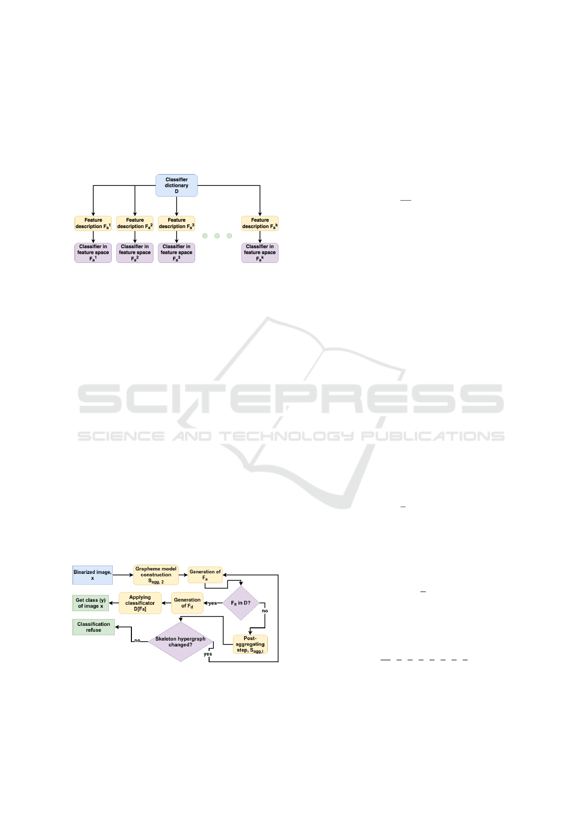
2. For each unique top-level feature F

, select the

objects that have this feature F

. For each of these

objects construct a bottom-level feature F

. As

the result a new subsample of objects from the F

feature space is selected, with which the classiﬁer

is trained (see Fig. 8).

Figure 8: Classiﬁcation dictionary D structure.

5.8 Classiﬁcation Algorithm

Let we have a new object x (binary image of a single

character), and it must be classiﬁed. To classify it, the

following steps are needed:

1. The selection of a mathematical model of grap-

heme S

agg,2

from x.

2. Building top-level features F

from S

agg,2

3. Check if F

in the classiﬁcation dictionary D, that

is obtained at the training stage. If the feature is

not present, the operation of postprocessing of the

skeleton graph is performed. If it is present then

skip to the next step.

4. The construction of bottom-level feature F

, the

application to it of the corresponding trained clas-

siﬁer and receiving a response.

The idea of post-processing is as follows: conti-

nuation of the search of the subgraph, which may be

classiﬁed according to the trained classiﬁcation dicti-

onary D. If such a graph was not found, the classiﬁ-

cation rejection will be returned

The ﬁnal algorithm can be seen in Fig. 9.

Figure 9: Binarized image classiﬁcation algorithm.

5.9 Quality Metric

Classiﬁcation accuracy is used as a quality metric.

Let a be a classiﬁcation algorithm, (X

, Y

) —

test sample, |X

| = n

, X

— i-th test sample object,

— its true class. Then the classiﬁcation accuracy

is calculated from the test sample according to the fol-

lowing formula:

Q(a, (X

, Y

)) =

∑

i=1

I[Y

= a(X

)].

6 COMPUTATIONAL

EXPERIMENTS

6.1 Training Dataset

For constructing a training dataset 88 different fonts

were selected, 33 letters of the Russian alphabet in lo-

wercase and uppercase versions (that is, only 66 grap-

hemes) in three font sizes were generated from each:

30, 50, 100 pixels. Image generation was performed

without smoothing, that is, immediately in binary for-

mat. The training sample size (X

, Y

) is n

= 17424

binarized letter images. As a true class Y

for the ob-

ject X

of the training dataset the letter in lowercase

was taken.

6.2 Parameters of the Proposed

Algorithm

1. Parameter of clipping is α = 0.06 · B

2. Threshold for trimming by length:

L(B) =

max(B

, B

3. The trimming threshold for length at the post-

processing stage increases in 1.8 times:

(B) = 1.8 · L(B) (κ = 1.8).

4. The trimming threshold for angle:

A =

5. At the stage of extraction of top-level features n =

m = 3 is supposed.

6. The ﬁxed grid is assumed to be equal to:





7. As classiﬁers at bottom-level is considered

Random forest (Ho, 1995).

VISAPP 2019 - 14th International Conference on Computer Vision Theory and Applications

356

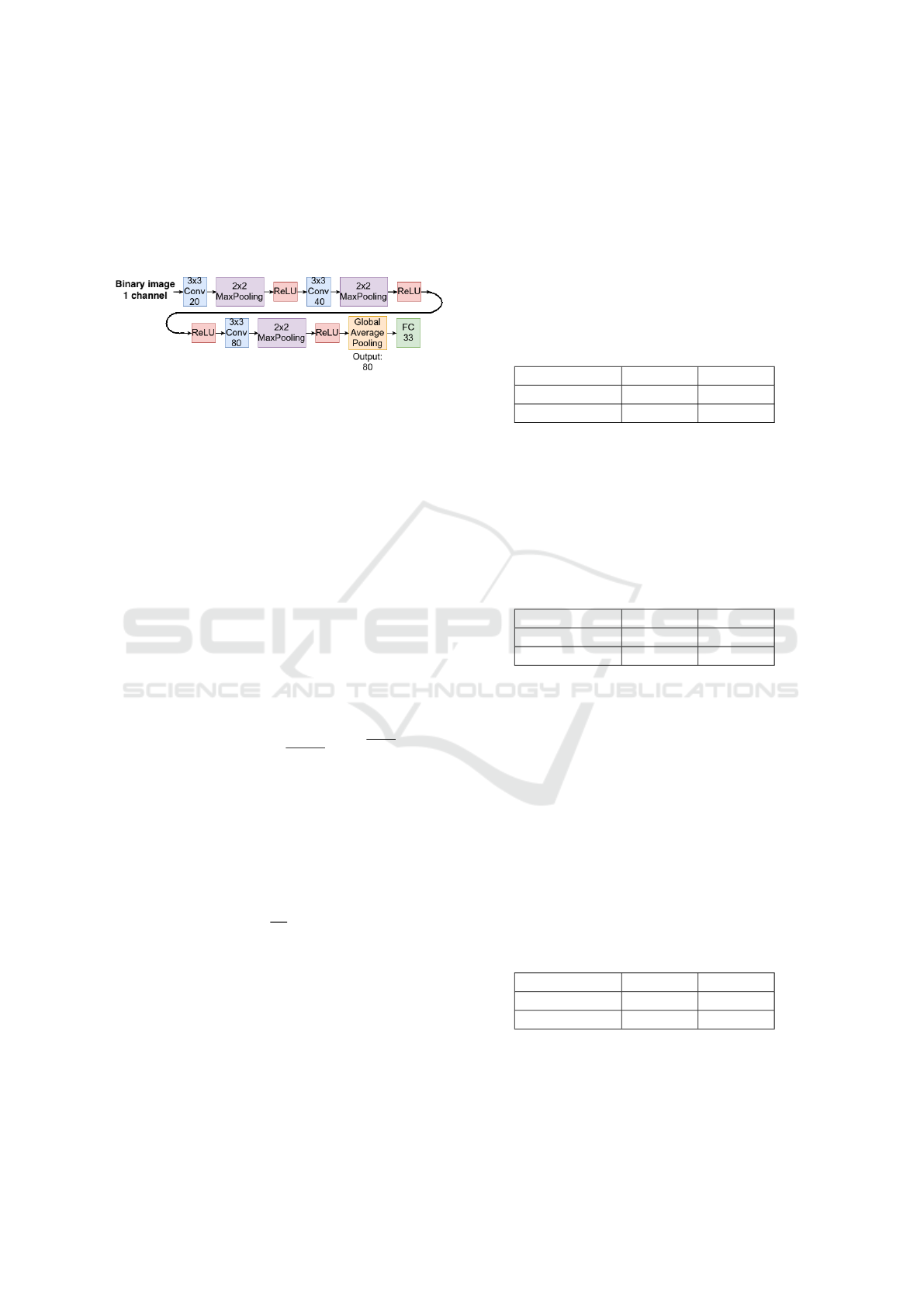
6.3 Basic Algorithm

As the base algorithm (baseline) has been selected

convolutional neural network (CNN) (LeCun et al.,

1998)(Bishop, 2006), the architecture of which is

shown in Fig. 10:

Figure 10: Neural network architecture.

Decoding of designations:

• k × k Conv f — convolution layer with kernel of

size k × k and f output ﬁlters (channels);

• k ×k MaxPooling — max-pooling layer with ker-

nel of size k × k;

• ReLU — ReLU layer (Glorot et al., 2011), (Jarrett

et al., 2009);

• Global Average Pooling — global average-

pooling layer (Lin et al., 2013);

• FC (Fully Connected) m — a fully connected

layer with an output layer of m neurons (Bishop,

2006).

For reasons of solving the classiﬁcation pro-

blem over the output layer (x

, x

, . . . , x

), softmax-

activation is performed from 33 neurons:

= softmax(x

) =

∑

j=1

, j = 1, 33.

Let C be a number of classes in the classiﬁcation

problem. Cross-entropy is taken here as the optimized

loss function.

L(y

, ˆy

) = −

∑

j=1

log ˆy

L(Y

, ˆy) =

∑

i=1

L(y

, ˆy

where ˆy

∈ [0, 1]

— prediction of the network on

i-th object, ˆy — prediction of the network on the entire

training dataset, y

— vector describing the observed

value: y

∈ [0, 1]

∑

j=1

= 1 and if i-th object has

class j (i.e. Y

= j) then y

= 1.

Remark. Since the input images can be of different

sizes, at the training stage the data in the neural net-

work was supplied by a batch consisting of 1 image.

6.4 Experiment 1

As a test dataset, the same 88 fonts that were used

in the training were taken, but a different font size,

which is 80 pixels. So n

= 5800. Images of letters

are generated using the program, that is, high-quality

images, without noise and binarized. The results of

two methods (structural analysis (SA) is the recogni-

tion method described in the article) are presented in

the table 1:

Table 1: The results of the two methods.

SA CNN

Quality, Q 0.99689 0.99862

Refusal rate 0.00086 0

6.5 Experiment 2

The test dataset consists of 50 fonts that were not used

when learning (FontsDatabase, 2018). The font size is

80 pixels, n

= 3300. Images of letters are generated

using the program. The results are presented in the

table 2:

Table 2: The results of the two methods.

SA CNN

Quality, Q 0.97 0.96515

Refusal rate 0.01364 0

6.6 Experiment 3

The test dataset consists of the same 50 fonts as in the

previous 6.5 experiment, and the same size. First, the

document is generated (.doc) with all the letters from

the test sample, then this document is converted into a

.png image with a resolution of 300 dpi. The images

from the RGB color representation were converted to

gray tones Y by the formula:

Y = 0.299R + 0.587G + 0.114B.

The images were then binarized using the Otsu

method (Otsu, 1979).

The results are presented in the table 3:

Table 3: The results of the two methods.

SA CNN

Quality, Q 0.94818 0.94454

Refusal rate 0.01485 0

6.7 Experiment 4

In this experiment, 18 sampled fonts from 50 fonts

of the 6.5 experiment are taken as a test dataset. The

Grapheme Approach to Recognizing Letters based on Medial Representation

357

font size is assumed to be 80 pixels, n

= 1188. The

document is generated (.doc) with all the letters from

the test sample, then this document is printed. Then

the obtained samples are scanned with a resolution of

300 dpi. That is, the images are of lower quality than

in the previous case (see Fig. 11).

Figure 11: Example letter from the input image

The results are presented in the table 4:

Table 4: The results of the two methods.

SA CNN

Quality, Q 0.95538 0.94696

Refusal rate 0.01263 0

6.8 Analysis of Experiments

The experiments show that: the quality of the propo-

sed method is not worse than the selected basic algo-

rithm and it has a small proportion of refuses from the

classiﬁcation, which increases with the deterioration

of image quality.

7 CONCLUSIONS

This paper proposes a formalization of the concept of

”grapheme”, namely a mathematical model of grap-

heme.

On the basis of this model, a method of genera-

ting features used for the subsequent construction of

the algorithm of classiﬁcation of images of letters is

proposed (that is, the measure of similarity between

mathematical models of graphs is determined). Also

in this article the algorithm of recognition of the text

on the image is proposed.

The advantages of the proposed letters recognition

method: independence from the size, type of font and

type of lettering; allocation of the general structure

(mathematical model of grapheme) for letters, which

is enough to recognize letters in new fonts; interpre-

tability of features.

The disadvantages of the method: the presence of

refuses of classiﬁcation and the dependence of the re-

cognition quality from the quality of the binarization

of the image.

The experiments conﬁrm that the proposed mat-

hematical model of the grapheme has shown its efﬁ-

ciency.

The objectives of further research are:

1. Improvement of top-level and bottom-level featu-

res.

2. Solution to the problem of classiﬁcation refuses.

3. Modiﬁcation of the iterative part (postprocessing)

of the classiﬁcation algorithm.

ACKNOWLEDGEMENTS

The work was funded by Russian Foundation of Basic

Research grant No. 17- 01-00917.

REFERENCES

Bishop, C. (2006). Pattern recognition and machine lear-

ning. Springer.

FontsDatabase (2018). https://www.fontsquirrel.com/.

Glorot, X., Bordes, A., and Bengio, Y. (2011). Deep sparse

rectiﬁer neural networks. In Proceedings of the four-

teenth international conference on artiﬁcial intelli-

gence and statistics, pages 315–323.

Hausdorff, F. (1965). Grundz

uge der mengenlehre (reprint;

originally published in leipzig in 1914). Chelsea, New

York.

Ho, T. K. (1995). Random decision forests. In Docu-

ment analysis and recognition, 1995., proceedings of

the third international conference on, volume 1, pages

278–282. IEEE.

Jarrett, K., Kavukcuoglu, K., LeCun, Y., et al. (2009). What

is the best multi-stage architecture for object recogni-

tion? In Computer Vision, 2009 IEEE 12th Internati-

onal Conference on, pages 2146–2153. IEEE.

LeCun, Y., Bottou, L., Bengio, Y., and Haffner, P. (1998).

Gradient-based learning applied to document recogni-

tion. Proceedings of the IEEE, 86(11):2278–2324.

Lin, M., Chen, Q., and Yan, S. (2013). Network in network.

arXiv preprint arXiv:1312.4400.

Mestetskiy, L. M. (2009). Continuous morphology of bi-

nary images: ﬁgures, skeletons, circulars (In Rus-

sian). FIZMATLIT.

Osetrova, O. V. (2006). Semiotics of the font (In Rus-

sian). Bulletin of Voronezh state University. Se-

ries:Philology. Journalism.

Otsu, N. (1979). A threshold selection method from gray-

level histograms. IEEE transactions on systems, man,

and cybernetics, 9(1):62–66.

ParaType (2008). Digital Fonts (In Russian). ParaType.

Solomonik, A. (2017). About language and languages (In

Russian). Publishing House ’Sputnik+’.

Zaliznyak, A. A. (2002). Russian nominal inﬂection by ap-

plication of selected works on modern Russian lan-

guage and General linguistics (In Russian). languages

of Slavic culture.

VISAPP 2019 - 14th International Conference on Computer Vision Theory and Applications

358