
Spatial Kernel Discriminant Analysis: Applied for Hyperspectral Image
Classification
Soumia Boumeddane
1
, Leila Hamdad
1
, Sophie Dabo-Niang
2
and Hamid Haddadou
1
1
Laboratoire de la Communication dans les Syst
`
emes Informatiques, Ecole nationale Sup
´
erieure d’Informatique,
BP 68M, 16309, Oued-Smar, Algiers, Algeria
2
Laboratoire LEM, Universit
´
e Lille 3, Lille, France
Keywords:
Kernel Density Estimation, Kernel Discriminant Analysis, Spatial Information, Supervised Classification.
Abstract:
Classical data mining models relying upon the assumption that observations are independent, are not suitable
for spatial data, since they fail to capture the spatial autocorrelation. In this paper, we propose a new super-
vised classification algorithm which takes into account the spatial dependency of data, named Spatial Kernel
Discriminant Analysis (SKDA). We present a non-parametric classifier based on a kernel estimate of the spa-
tial probability density function which combines two kernels: one controls the observed values while the other
controls the spatial locations of observations. We applied our algorithm for hyperspectral image (HSI) classi-
fication, a challenging task due to the high dimensionality of data and the limited number of training samples.
Using our algorithm, the spatial and spectral information of each pixel are jointly used to achieve the classi-
fication. To evaluate the efficiency of the proposed method, experiments on real remotely sensed images are
conducted, and show that our method is competitive and achieves higher classification accuracy compared to
other contextual classification methods.
1 INTRODUCTION
Most statistical and machine learning methods as-
sume that data samples are independent and identi-
cally distributed (i.i.d.). This assumed pre-condition
about the independence of observations is not verified
when dealing with spatial data (Cheng et al., 2014a)
captured in many fields such as ecology, image analy-
sis, epidemiology and environmental science. In fact,
spatial data are characterized by spatial autocorrela-
tion or spatial dependency phenomenon. This charac-
teristic is defined as the tendency of near observations
to be more similar than distant observations in space
(Cheng et al., 2014b). This property is formulated as
the first law of geography : ”Everything is related to
everything else, but near things are more related than
distant things” (Tobler, 1970). For example, measure-
ments taken in neighboring sites are more likely to
be similar then those of distant locations, natural phe-
nomena vary gradually over space and objects of sim-
ilar characteristics tend to be clustered (ex: popula-
tion with similar socio-economic characteristics and
preferences,...etc) (Shekhar et al., 2009).
Ignoring this property of autocorrelation when an-
alyzing spatial data may lead to inaccurate or incon-
sistent models or hypotheses (Shekhar et al., 2015),
produce biased discriminant rules (Bel et al., 2009),
hide important insight and could even invert patterns
(Stojanova et al., 2013). An effective analysis of spa-
tial data must take into account geographic positions
of observations and the existing relationship due to
their proximity.
Several supervised learning methods modeling
spatial dependency for classification and regression
are considered in the literature: Markov Random
Field-based Bayesian classifiers, which integrates the
spatial information of data via the a priori term in
Bayes rule ; The logistic spatial autoregression (SAR)
model, which models the spatial dependence directly
in the regression equation using a neighborhood rela-
tionship contiguity matrix and a weight of the spa-
tial dependency; and Geographically Weighted Re-
gression (GWR) which includes a spatial variation pa-
rameter in regression equation (Shekhar et al., 2011).
More recently, (Stojanova et al., 2013) proposed
SCLUS (Spatial Predictive Clustering System), a pre-
dictive clustering tree framework that learn from spa-
tial autocorrelated data .
Various indices are proposed to measure the spa-
tial autocorrelation, from a global or a local point of
184
Boumeddane, S., Hamdad, L., Dabo-Niang, S. and Haddadou, H.
Spatial Kernel Discriminant Analysis: Applied for Hyperspectral Image Classification.
DOI: 10.5220/0007372401840191
In Proceedings of the 11th International Conference on Agents and Artificial Intelligence (ICAART 2019), pages 184-191
ISBN: 978-989-758-350-6
Copyright
c
2019 by SCITEPRESS – Science and Technology Publications, Lda. All rights reserved

view, such as : Moran’s I index, c index of Geary,
Cliff and Ord indices, Getis and Ord (G
i
et G
∗
i
) indices
and Local Indicators of Spatial Association (LISA)
(Shekhar et al., 2015).
We focus in this work on supervised classification
task. We propose a new classification algorithm for
spatially autocorrelated data, that we call SKDA, for
Spatial Kernel Discriminant Analysis. Our algorithm
is a spatial extension of classical Kernel Discriminant
Analysis rule; it is founded on a kernel estimate of
the spatial probability density function that integrates
two kernels: one controls the observed values while
the other controls the spatial locations of observations
(Dabo-Niang et al., 2014).
One potential application of our SKDA algo-
rithm is the classification of remotely sensed hy-
perspectral images. This problem has attracted a
lot of attention over the past decade. Several stud-
ies proposed spectral-spatial classification algorithms
which integrate spatial context and spectral infor-
mation of the hyperspectral image. This incorpo-
ration of spatial information has shown great im-
pact for improving classification accuracy (He et al.,
2017). According to the way the spatial dimension
is incorporated, these methods can be classified into
three main categories: integrated spectral-spatial ap-
proaches, preprocessing-based approaches, and post-
processing-based approaches (Fauvel et al., 2013). A
survey about the incorporation of spatial information
for HSI classification is presented in (Wang et al.,
2016).
The contribution of our work is double; on one
hand, we propose a spatial classification algorithm
managing the dependency of data, on the other hand,
a spatial-spectral method is proposed for the classifi-
cation of HSI with competitive results.
The remainder of the paper is organized as fol-
lows: Section 2 defines the context of this study, and
presents the background knowledge essential to the
understanding of our algorithm. Section 3 presents
our SKDA algorithm. Section 4 shows experimental
results of our method on hyperspectral image classi-
fication. Finally, section 5 summarizes the results of
this work and draws conclusions.
2 BACKGROUND
In this section, we begin by formally defining the nec-
essary notations that we will adopt throughout this pa-
per. Then, present the background knowledge essen-
tial to the understanding of our algorithm.
In this work, we focus on geostatistical data, we
consider a spatial process {Z
i
= (X
i
,Y
i
) ∈ R
d
× N,i ∈
Z
N
,d ≥ 1,N ∈ N
∗
}, defined over a probability space
(Ω,F,P) and indexed in a rectangular region I
n
= {i ∈
Z
N
: N ∈ N
∗
,1 ≤ i
k
≤ n
k
,∀k ∈ {1, ...,N}}. Where a
point i = (i
1
,...,i
N
) ∈ Z
N
is called a site, representing
a geographic position. And let ˆn = n
1
×n
2
×...×n
N
=
Card(I
n
) be the sample size, and f(.) the density func-
tion of X ∈ R
d
. Each site i ∈ I
n
is characterized by a
d-dimensional observation x
i
= (x
i1
,x
i2
,...,x
id
).
In this work we are interested on supervised clas-
sification which consists of building a classifier that
from a given training set containing input-output pairs
allows to predict a class Y
i
∈ {1, 2,..., m} of a new ob-
servation x
i
.
2.1 Bayes Classifier
Bayes classifier is one of the widely used classifica-
tion algorithms due to its simplicity, efficiency and
efficacy. It is a probabilistic classifier which rely on
Bayes’ theorem and the assumption of independence
between the features, in other words, the classification
decision is made basing on probabilities. It consist of
assigning an instance x to the class with the highest a
posteriori probability.
Supposing that we have m classes, associated each
with a probability density function f
k
where f
k
=
P(x/k) and an a priori probability π
k
that an obser-
vation belongs to the class k, k ∈ {1,2,..., m}. Bayes
discriminant rule is formulated as follows :
Assign x to class k
0
where k
0
= arg
max
k∈{1,2,...,m}
(π
k
f
k
(x))
(1)
2.2 Kernel Density Estimation
As we might notice, Bayesian methods require a
background knowledge of many probabilities, which
consists of a practical difficulty to apply it. To avoid
these requirements, these probabilities can be esti-
mated based on available labeled data or by mak-
ing assumptions about the distributions (Gramacki,
2018). Two classes of density estimators are recog-
nized in the literature. The first, known as paramet-
ric methods are based upon the assumption that data
are drawn form an arbitrary well known distribution
(e.g. Gaussian, Gamma, Cauchy ... etc.) and finding
the best parameters describing this distribution . Two
commonly used techniques can be sited: Bayesian pa-
rameter estimation and maximum likelihood. How-
ever, this assumption about the form of the under-
lying density is not always possible because of the
complexity of data. In such cases, nonparametric es-
timation techniques are required. These methods do
not make any a priori assumptions about the distri-
Spatial Kernel Discriminant Analysis: Applied for Hyperspectral Image Classification
185

bution but estimate the density function directly from
the data (Gramacki, 2018).
One of the most known non-parametric density
estimation techniques is Kernel Density Estimation
(KDE). First contributions concerning kernel estima-
tion of (Parzen, 1962) and (Rosenblatt, 1985) for spa-
tial densities are due to (Tran, 1990). A marginal den-
sity of a point x ∈ R
d
is defined as :
ˆ
f (x) =
1
ˆnh
d
∑
i∈I
n
K
x − X
i
h
,x ∈ R
d
(2)
Where h is a smoothing parameter called band-
width and K is a weight function, called ”kernel”
which decreases as the distance between x and X
i
in-
creases. This function satisfies the following condi-
tion:
Z
+∞
−∞
K(x) dx = 1 (3)
Different kernel functions have been proposed in
the literature: Uniform, Triangle, Epanechnikov ...
etc.
KDE is a relevant tool for analyzing and visualiz-
ing the distribution of spatial process. Moreover, it is
one of the most common methods for hotspots map-
ping, used for crash and crimes data (Chainey et al.,
2008).
2.3 Kernel Discriminant Analysis
Replacing class densities f
i
in Bayes discriminant rule
(Equation 1) by its kernel density estimate given in
Equation 2 , define a new classifier known as Ker-
nel Discriminant Rule , the base of Kernel Discrimi-
ant Analysis supervised algorithm. According to Ker-
nel Discriminant Rule, an observation x ∈ R
d
will be
assigned to the group k
0
which maximize
ˆ
π
k
ˆ
f
k
(x) .
Where
ˆ
π
k
is an estimator of the a priori probabilities
π
k
, given by
ˆ
π
k
=
m
k
ˆn
(4)
and m
k
is the size of the k-th class.
2.4 Spatial KDE
Kernel density estimator previously presented does
not take into account spatial autocorrelated data. In
fact, to estimate a density at a site, all the data points
are used and no specific weight is given to neighbor-
ing sites. In (Dabo-Niang et al., 2014), the authors
proposed a kernel density estimation of a spatial den-
sity function, which incorporates spatial dependency
of data. They propose a new version of (Tran, 1990)
estimator (Equation 2) which has the particularity of
taking into account not only the values of the obser-
vations but also the position of sites where the obser-
vations occurred. They established its uniform almost
sure convergence and they studied the consistency of
its mode. They proposed a spatial density estimation
of a discretely indexed spatial process i.e. a random
field (X
i
,i ∈ Z
N
,N > 1), with values in R
d
,d ≥ 1 and
defined over a probability space (Ω,F,P).
For each observation x
j
∈ R
d
located at a site j ∈
I
n
, this spatial density estimator is defined as follows:
ˆ
f (x
j
) =
1
ˆnh
d
v
h
N
s
∑
i∈I
n
K
1
x
j
− X
i
h
v
K
2
ki − jk
h
s
(5)
Where
• h
v
and h
s
are two bandwidths controling observa-
tions (values) and sites position respectively,
• K
1
and K
2
are two kernels respectively defined in
R
d
and R, where the first manage observation val-
ues while the second deals with spatial locations
of these observations.
• And k i − j k is the euclidean distance between
sites i and j .
In the case where I
n
is a rectangular grid i.e. N = 2
, Equation 5 become;
ˆ
f (x
j
) =
1
ˆnh
d
v
h
2
s
∑
i∈I
n
K
1
x
j
− X
i
h
v
K
2
ki − jk
h
s
(6)
The incorporation of a second kernel K
2
allows
this estimator to give a weight to sites, which de-
crease as the distance between corresponding sites
increases. Consequently, to estimate f (x
j
) at a site
j, only the neighboring sites are considered because
they can bring sufficient information about the distri-
bution of X
j
, which means that the farther a site i is
from j, the lower is the dependence between X
i
and
X
j
. More details about this estimator can be found in
(Dabo-Niang et al., 2014).
3 SPATIAL KERNEL
DISCRIMINANT ANALYSIS
In what follows, we propose a novel supervised spa-
tial classification algorithm allowing a classification
of an observation at a new site, based not only on the
observation itself but taking in consideration the posi-
tion of sites. In other words, the classification is based
on the observations of neighboring sites. The totality
of data is exploited to achieve the classification: the
value of the observation, the position of the new site
and training model from the nearby sites.
ICAART 2019 - 11th International Conference on Agents and Artificial Intelligence
186

We present a new kernel discriminant rule for
strongly mixing random fields, which means that sites
located at a proximity are more dependent than distant
sites. Thus, if a distance between two sites is high,
their values are independent and it is more likely that
they belongs to different classes.
Our classification rule consists of assigning a new
observation x ∈ R
d
at a site i
0
to the class k
0
where
k
0
= arg
max
k∈{1,2,...,m}
(
ˆ
π
k
ˆ
f
k
(x))
Where
ˆ
π
k
is estimated as follow:
ˆ
π
k
=
m
k
ˆ
N
(7)
Suppose that X
k1
,X
k2
,...,X
kmk
are d-dimensional ob-
servations from the k-th class, spatial Kernel Density
estimate is defined as follows (based on (Dabo-Niang
et al., 2014) estimator):
ˆ
f
k
(x
j
) =
1
m
k
h
d
v
h
2
s
∑
i∈I
n
,
C(X
ki
)=k
K
1
x
j
− X
ki
h
v
K
2
ki − jk
h
s
(8)
Where
• C(.) is the class label of an observation,
• m
k
is the size of k-th class in the training data
•
ˆ
N is the size of the training set
The kernel function K
1
is a multivariate kernel with
values in R
d
. In this work, we suggest to define this
kernel as a multiplicative kernel, as follows:
For X = (x
1
,x
2
,...,x
d
) in R
d
:
K
1
(X) = K(x
1
) × K(x
2
) × ... × K(x
d
) (9)
Where: K is a univariate Kernel. More specifically:
K
1
x
j
− X
i
h
v
= K
x
j1
− X
i1
h
v
× ...×
x
jd
− X
id
h
v
=
d
∏
l=1
K
x
jl
− X
il
h
v
We summarize in Algorithm 1 the main steps of
our SKDA technique. We precise that, in order to de-
crease the execution time of our algorithm, the term
K
1
(.) in Equation 8 is computed only when the term
K
2
(.) 6= 0. In addition, for a testing set, step 2 in Al-
gorithm 1, is executed one time.
Algorithm 1: Spatial Kernel Discriminant Analysis
algorithm.
Result:
• Classfication of an observation at a new site
Input :
• X
i0
: an observation to be classified, situated at a
site i
0
• A set of training data (X
i
,y
i
) ∈ R
d
× {1,2,.., m},
where y
i
is the class label of X
i
Output:
• k
0
: the class label of X
i0
1 foreach class k ∈ {1,2, ..., m} do
2 Compute a priori probability
ˆ
π
k
(using
Equation 7)
3 Compute
ˆ
f
k
(x
i0
) using Equation 8, based on
learning data of the k-th class
4 end
5 k
0
= arg
max
k∈{1,2,...,m}
(
ˆ
π
k
ˆ
f
k
(x))
4 EXPERIMENTAL RESULTS
4.1 Hyperspectral Images Classification
One potential application of our algorithm on real
data would be the classification of remotely sensed
hyperspectral images. A hyperspectral image (HSI)
is a set of simultaneous images collected for the same
area on the surface of the earth with hundreds of spec-
tral bands at different wavelength channels and with
high resolution (He et al., 2017). A HSI is represented
as a hyperspectral cube with spectral and spatial di-
mension (Figure 1). Each pixel is described by its po-
sition and a spectral vector, where its size correspond
to the number of spectral bands collected by the sen-
sor (Fauvel et al., 2013).
Hyperspectral image classification consists of as-
signing a unique label to a pixel vector, representing
a thematic class such as forest, urban, water, and agri-
culture. These images are considered as a relevant
tool for many applications, such as ecology, geology,
hydrology, precision agriculture, and military appli-
cations (Ghamisi et al., 2017).
Using our classification algorithm in this context
is considered as spectral-spatial classification tech-
nique which exploits all information available in an
HSI to achieve better accuracy of classification.
Spatial Kernel Discriminant Analysis: Applied for Hyperspectral Image Classification
187

Figure 1: Hyperspectral image representation.
4.2 Data Set
In order to evaluate and validate the effectiveness of
our method, we carried out experiments on a widely
used real-world hyperspectral image dataset: the In-
dian Pines benchmark
1
. The scene represents Pine
forests of Northwestern Indiana in America in 1992.
This data set is a very challenging land-cover classi-
fication problem, due to the presence of mixed pixels
(Appice et al., 2017) and the non-proportionality be-
tween the size of different classes. In addition, the
crops (mainly corn and soybeans) of this scene are
captured in early stages of growth with less than 5%
coverage, which makes discrimination between these
crops a difficult task.
This scene was captured using NASA’s Airborne
Visible/Infrared Imaging Spectrometer (AVIRIS) sen-
sor, with a size of 145 × 145 pixels, classified into
16 ground-truth land-cover classes, where each class
contains from 20 to 2468 pixels. The effective size
of this dataset is 10249 pixels after removing the im-
age background (pixels with a label equal to zero).
Each pixel is characterized by 200 spectral bands, af-
ter eliminating 20 noisy channels corresponding to the
water absorption bands. The color composite image
and the corresponding ground truth map are shown in
Figure 2.
Due to the expensive cost of manual labeling of
hyperspectral images pixels, the number of training
samples is often limited, this represent a challeng-
ing task for classification algorithms (Ghamisi et al.,
2017). Thus, our SKDA algorithm should be capable
to well-perform even if only a few labelled samples
are available. To build the training set, we randomly
selected only 10% of pixels from each class, and the
remaining pixels forms the test set.
1
Available on www.ehu.eus/ccwintco/index.php/
Hyperspectral Remote Sensing Scenes
Figure 2: Indian Pines image. (a) Three-band color com-
posite. (b) Reference data. (c) Color code.
Table 1: Class labels and the number of training and testing
samples for Indian pines.
- Class Train Test Total
1 Alfalfa 4 42 46
2 Corn-no till 142 1286 1428
3 Corn-min till 83 747 830
4 Corn 23 214 237
5 Grass-pasture 48 435 483
6 Grass-trees 73 657 730
7 Grass-pasture-
mowed
2 26 28
8 Hay-windrowed 47 431 478
9 Oats 2 18 20
10 Soybean-no till 97 875 972
11 Soybean-min till 245 2210 2455
12 Soybean-clean 59 534 593
13 Wheat 20 185 205
14 Woods 126 1139 1265
15 Build-Grass-
Trees-Drives
38 348 386
16 Stone-Steel-
Towers
9 84 93
Total 1018 9231 10249
Table 1 shows the size of training and testing sets
of each class of Indian Pines scene.
4.3 Performance Comparison
To evaluate the performance of our algorithm com-
pared to other methods, we employ three widely used
classification accuracy measures: Overall accuracy
(OA), Average Accuracy (AA) and per class accuracy.
ICAART 2019 - 11th International Conference on Agents and Artificial Intelligence
188
OA is defined as the ratio between the number of well-
classified pixels to the size of testing set, while AA is
the average of per-class classification accuracies.
The results of classification depends on the train-
ing and testing sets which are randomly selected. To
reduce this effect and make the comparison fair, we
repeat each experiment 10 times with different train-
ing and testing sets and we report the mean accuracy
of these executions. We use Epanechnikov Kernel
for the two kernels K
1
and K
2
with observation band-
width h
v
equal to 700 and a spatial bandwidth h
s
of 3.
We obtained these optimal values of h
v
and h
s
band-
widths by studying their influence on overall and av-
erage classification accuracies. In fact, we varied em-
pirically the values of these two bandwidth, and select
the combination which gave the highest OA and AA.
In this section, we present the quantitative results
achieved by our SKDA algorithm and the results of
nine different methods reported from (Zhou et al.,
2018). To have a fair comparison we use the same
ratio of training and testing set as this work. Tables 2
shows the classification accuracy for each class, over-
all accuracy (OA) and average accuracy (AA), where
the best accuracies are in bold.
Table 2 demonstrates that our proposed SKDA al-
gorithm outperforms other methods, with an improve-
ment of Average Accuracy by 5,58%, the Overall Ac-
curacy by 3,04% and per-class accuracy till 16,11%
(expect for Wheat class) comparing to SSLSTMs ap-
proach.
It can be observed that spectral-spatial approaches
(MDA, CNN, LSTM-based methods and SKDA)
gives significantly better accuracies then pixel-wised
methods (PCA, LDA, NWFE, RLDE) which are
based only on observations values.
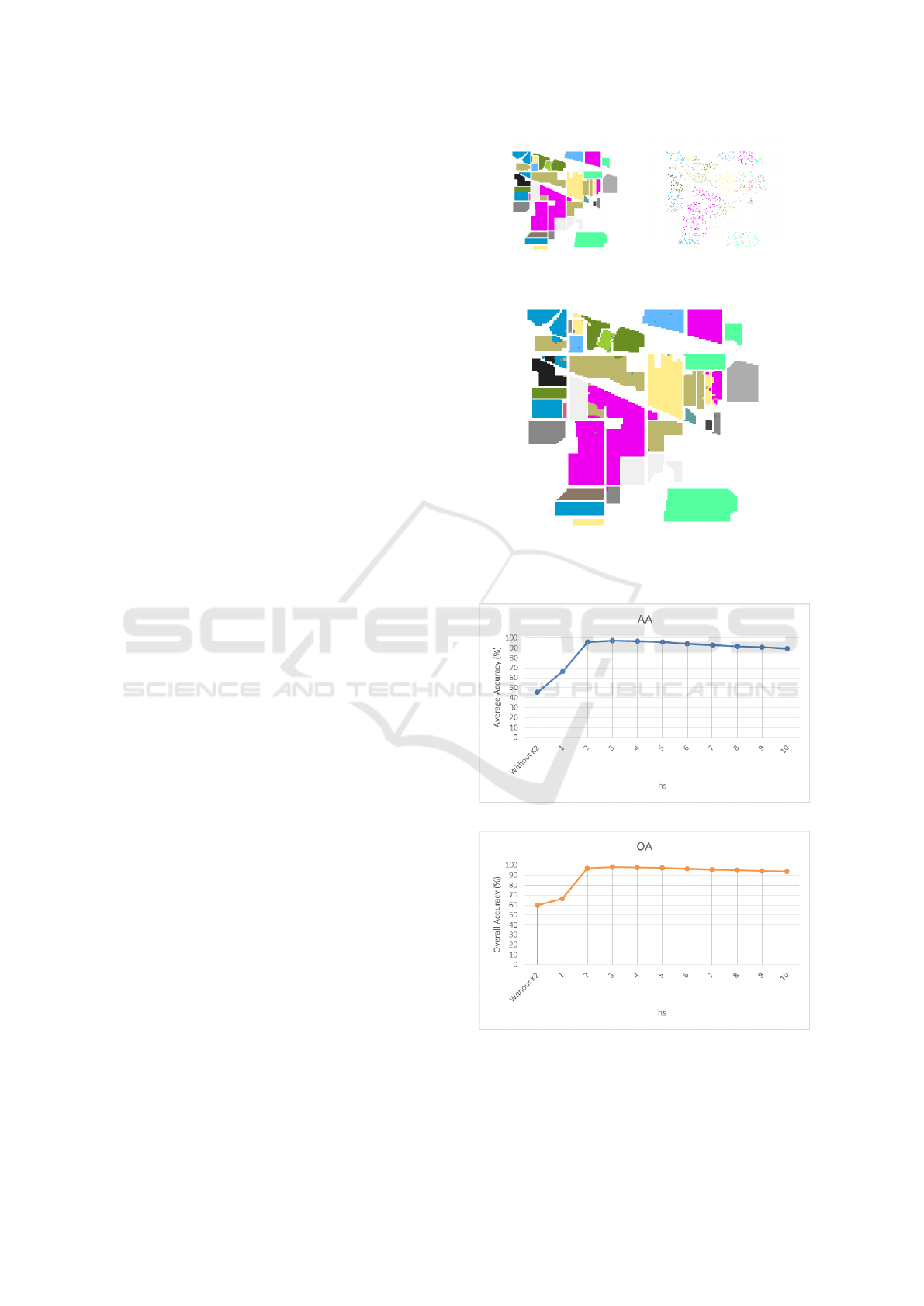
Figure 3 visualize the classification result of In-
dian pines data set using our SKDA algorithm and the
training data used for density estimation.
4.4 Influence of Parameters
Our classification algorithm depends on two band-
widths: h
v
and h
s
, that control observation values and
spatial neighborhood respectively. In this section, we
analyze the impact of the integration of the spatial di-
mension of data in the classification process through
the study of the influence of the spatial bandwidth h
s
on overall and average accuracies. We set the value
of the bandwidth h
v
to 700, and we vary h
s
from 1 to
10 and compare the results also with classical version
of Kernel Discriminant Analysis that don’t take into
account the spatial context of data (the estimation of
density is based only on the values of observations i.e
the second kernel K
2
is not used).
(a) Indian Pines dataset (b) Training set
(c) SKDA classification result, h
v
= 700, h
s
= 3
Figure 3: Classification visualisation.
(a) The effect of hs bandwidth on AA.
(b) The effect of hs bandwidth on OA.
Figure 4: Influence of spatial bandwidth.
Spatial Kernel Discriminant Analysis: Applied for Hyperspectral Image Classification
189

Table 2: Classification accurracy (%) for Indian Pines data set.
Label PCA LDA NWFE RLDE MDA CNN SeLSTM SaLSTM SSLSTMs SKDA
OA 72.58 76.67 78.47 80.97 92.31 90.14 72.22 91.72 95.00 98.04
AA 70.19 72.88 76.08 80.94 89.54 85.66 61.72 83.51 91.69 97.27
1 59.57 63.04 62.17 64.78 73.17 71.22 25.85 85.85 88.78 98.57
2 68.75 72.04 76.27 78.39 93.48 90.10 66.60 89.56 93.76 96.88
3 53.95 57.54 59.64 68.10 84.02 91.03 54.83 91.43 92.42 96.59
4 55.19 46.58 59.83 70.80 83.57 85.73 43.94 90.61 86.38 96.77
5 83.85 91.76 88.49 92.17 96.69 83.36 83.45 88.60 89.79 96.78
6 91.23 94.41 96.19 94.90 99.15 91.99 87.76 90.81 97.41 99.75
7 82.86 72.14 82.14 85.71 93.60 85.60 23.20 51.20 84.80 95.38
8 93.97 98.74 99.04 99.12 99.91 97.35 95.40 99.02 99.91 99.97
9 34.00 26.00 44.00 73.00 63.33 54.45 30.00 38.89 74.44 90.55
10 64.18 60.91 69.18 69.73 82.15 75.38 71.29 88.64 95.95 96.73
11 74.96 76.45 77.78 79.38 92.76 94.36 75.08 94.62 96.93 98.74
12 41.72 67.45 64.05 72.28 91.35 78.73 54.49 86.10 89.18 96.10
13 93.46 96.00 97.56 97.56 99.13 95.98 91.85 90.11 98.48 99.02
14 89.45 93.79 93.49 92.36 98.22 96.80 90.37 98.10 98.08 99.92
15 47.77 65.54 58.50 67.10 87.84 96.54 30.49 88.59 92.85 98.33
16 88.17 83.66 89.03 89.68 94.29 81.90 62.86 64.05 87.86 96.30
Figure 4 shows overall and average accuracies as
a function of h
s
bandwidth. This plot proves that the
integration of the spatial dimension of data improves
drastically the classification accuracy, and that the re-
sults obtained by our SKDA algorithm exceeds those
obtained by classical KDA. In fact, the AA increased
from 45% to 70% when spatial dependency is consid-
ered (when h
s
= 1). Best accuracies were obtained
when h
s
= 3, with an Average Accuracy of 97,27%
and an Overall Accuracy of 98,04% (as mentioned in
the previous section). However, when greater values
of h
s
are used, a degradation of OA and AA is cap-
tured.
This experiment proves that the choice of the spa-
tial bandwidth h
s
is crucial. In fact, small values
of this bandwidth are not sufficient for the learning
model; while, larger values decrease the classification
accuracy because they lead to an over-smoothing of
the density.
5 CONCLUSION
In this paper, a Kernel Discriminant Analysis algo-
rithm for spatial data named SKDA is proposed. This
supervised classification algorithm allows taking into
consideration the spatial autocorrelation of data, and
exploiting all the available information: the observa-
tions in one hand and their positions in other hand.
Another contribution of this work is the proposition
of a new spatial-spectral hyperspectral image classi-
fication algorithm. Experimental tests on real word
dataset shows that our SKDA algorithm outperforms
other contextual classification algorithms and proves
that the integration of the spatial dimension of data in-
creases the classification accuracy, even with limited
number of training samples and high-dimensionality
of data. Experiments on other hyperspectral images
benchmark datasets are ongoing. Moreover, we aim
to propose an efficient way for bandwidths tuning,
since the classification accuracy depends on.
REFERENCES
Appice, A., Guccione, P., and Malerba, D. (2017). A novel
spectral-spatial co-training algorithm for the transduc-
tive classification of hyperspectral imagery data. Pat-
tern Recognition, 63:229–245.
Bel, L., Allard, D., Laurent, J. M., Cheddadi, R., and Bar-
Hen, A. (2009). CART algorithm for spatial data: Ap-
plication to environmental and ecological data. Com-
putational Statistics & Data Analysis, 53(8):3082–
3093.
Chainey, S., Tompson, L., and Uhlig, S. (2008). The utility
of hotspot mapping for predicting spatial patterns of
crime. Security journal, 21(1-2):4–28.
Cheng, T., Haworth, J., Anbaroglu, B., Tanaksaranond, G.,
and Wang, J. (2014a). Spatiotemporal data mining.
In Handbook of regional science, pages 1173–1193.
Springer.
Cheng, T., Wang, J., Haworth, J., Heydecker, B., and Chow,
A. (2014b). A dynamic spatial weight matrix and lo-
calized space–time autoregressive integrated moving
average for network modeling. Geographical Analy-
sis, 46(1):75–97.
Dabo-Niang, S., Hamdad, L., Ternynck, C., and Yao, A.-
F. (2014). A kernel spatial density estimation allow-
ing for the analysis of spatial clustering. application
ICAART 2019 - 11th International Conference on Agents and Artificial Intelligence
190

to monsoon asia drought atlas data. Stochastic envi-
ronmental research and risk assessment, 28(8):2075–
2099.
Fauvel, M., Tarabalka, Y., Benediktsson, J. A., Chanussot,
J., and Tilton, J. C. (2013). Advances in spectral-
spatial classification of hyperspectral images. Pro-
ceedings of the IEEE, 101(3):652–675.
Ghamisi, P., Plaza, J., Chen, Y., Li, J., and Plaza, A. J.
(2017). Advanced spectral classifiers for hyperspec-
tral images: A review. IEEE Geoscience and Remote
Sensing Magazine, 5(1):8–32.
Gramacki, A. (2018). Nonparametric Kernel Density Esti-
mation and Its Computational Aspects. Springer.
He, L., Li, J., Plaza, A., and Li, Y. (2017). Discrimina-
tive low-rank gabor filtering for spectral-spatial hyper-
spectral image classification. IEEE Trans. Geoscience
and Remote Sensing, 55(3):1381–1395.
Parzen, E. (1962). On estimation of a probability density
function and mode. The annals of mathematical statis-
tics, 33(3):1065–1076.
Rosenblatt, M. (1985). Stationary sequences and random
fields.
Shekhar, S., Evans, M. R., Kang, J. M., and Mohan, P.
(2011). Identifying patterns in spatial information: A
survey of methods. Wiley Interdisc. Rew.: Data Min-
ing and Knowledge Discovery, 1(3):193–214.
Shekhar, S., Jiang, Z., Ali, R. Y., Eftelioglu, E., Tang, X.,
Gunturi, V. M. V., and Zhou, X. (2015). Spatiotempo-
ral data mining: A computational perspective. ISPRS
Int. J. Geo-Information, 4(4):2306–2338.
Shekhar, S., Kang, J., and Gandhi, V. (2009). Spatial data
mining. In Encyclopedia of Database Systems, pages
2695–2698. Springer.
Stojanova, D., Ceci, M., Appice, A., Malerba, D., and Dze-
roski, S. (2013). Dealing with spatial autocorrelation
when learning predictive clustering trees. Ecological
Informatics, 13:22–39.
Tobler, W. R. (1970). A computer movie simulating urban
growth in the detroit region. Economic geography,
46(sup1):234–240.
Tran, L. T. (1990). Kernel density estimation on random
fields. Journal of Multivariate Analysis, 34(1):37–53.
Wang, L., Shi, C., Diao, C., Ji, W., and Yin, D. (2016).
A survey of methods incorporating spatial informa-
tion in image classification and spectral unmixing. In-
ternational Journal of Remote Sensing, 37(16):3870–
3910.
Zhou, F., Hang, R., Liu, Q., and Yuan, X. (2018). Hy-
perspectral image classification using spectral-spatial
lstms. Neurocomputing.
Spatial Kernel Discriminant Analysis: Applied for Hyperspectral Image Classification
191
