An Optimized E-nose for Efﬁcient Volatile Sensing and Discrimination

Gonc¸alo Santos

1,∗

, Cl

audia Alves

, Ana Carolina P

adua

, Susana Palma

Hugo Gamboa

and Ana Cec

ılia Roque

UCIBIO, Departamento de Qu

ımica, Faculdade de Ci

encias e Tecnologia da Universidade NOVA de Lisboa,

2829-516 Caparica, Portugal

Laborat

orio de Instrumentac¸

ao Engenharia Biom

edica e F

ısica da Radiac¸

ao (LIBPhys-UNL), Departamento de F

ısica,

Faculdade de Ciencias e Tecnologia da Universidade NOVA de Lisboa, Monte da Caparica, 2829-516 Caparica, Portugal

Keywords:

Electronic Nose, Volatile Organic Compounds, Machine Learning, Biomaterials.

Abstract:

Electronic noses (E-noses), are usually composed by an array of sensors with different selectivities towards

classes of VOCs (Volatile Organic Compounds). These devices have been applied to a variety of ﬁelds, includ-

ing environmental protection, public safety, food and beverage industries, cosmetics, and clinical diagnostics.

This work demonstrates that it is possible to classify eleven VOCs from different chemical classes using a

single gas sensing biomaterial that changes its optical properties in the presence of VOCs. To accomplish this,

an in-house built E-nose, tailor-made for the novel class of gas sensing biomaterials, was improved and com-

bined with powerful machine learning techniques. The device comprises a delivery system, a detection system

and a data acquisition and control system. It was designed to be stable, miniaturized and easy-to-handle. The

data collected was pre-processed and features and curve ﬁtting parameters were extracted from the original

response. A recursive feature selection method was applied to select the best features, and then a Support

Vector Machine classiﬁer was implemented to distinguish the eleven distinct VOCs. The results show that the

followed methodology allowed the classiﬁcation of all the VOCs tested with 94.6% (± 0.9%) accuracy.

1 INTRODUCTION

The human olfactory system is sophisticated and is

able to detect spoiled food, to identify dangerous en-

vironments or pleasant experiences. Highly trained

humans can even develop this sense beyond the usual

limits. Hippocrates (430 B.C.), considered the father

of medicine, could diagnose diseases by smelling pa-

tient’s biological samples (R

ock et al., 2008). Odours

consist of sets of volatile organic compounds (VOCs).

When VOCs ﬂow through the human’s nasal cavity,

they reach the olfactory epithelium, where olfactory

sensory neurons deﬁne action potentials up their own

axons, until the olfactory bulb, which then transmits

the signal to the brain, where recognition occurs (Bar-

bosa et al., 2018).

The intriguing olfactory system has inspired re-

searchers to develop technologies mimicking natural

olfaction (Wasilewski et al., 2017; He et al., 2012;

adua et al., 2018b).

The best example of artiﬁcial olfaction is the con-

cept of electronic nose (E-nose). E-noses comprise

of an array of semi-selective sensors (e.g. metal ox-

ide semiconductor or MOS-based sensors, conduct-

ing polymers, piezoelectric quartz crystals) which

change properties in the presence of VOCs (Arshak

et al., 2004). Physico-chemical changes that occur in

the sensors during VOCs exposure are typically con-

verted to electrical signals by the transduction system.

The acquired data is further analysed and processed

andd VOC recognition is performed.

A set of features is ﬁrstly extracted and selected

from the signals obtained. (Yan et al., 2015) reviewed

many feature extraction methods, including features

extraction from the original response curves, curve

ﬁtting parameters and transform domains. As con-

clusion, the authors stated that the best method de-

pends on the situation. Nevertheless, some advice

was given: for steady-state features, normalization

models are the best option; transient features, such as

derivatives and integrals of original response curves,

have more information than steady-state features (Yan

et al., 2015).

After features selection, advanced computational

techniques can be applied. Examples of linear clas-

siﬁcation methods are principal component analysis

(PCA), linear discriminant analysis (LDA), functional

discriminant analysis (FDA), partial least square dis-

Santos, G., Alves, C., Pádua, A., Palma, S., Gamboa, H. and Roque, A.

An Optimized E-nose for Efﬁcient Volatile Sensing and Discrimination.

DOI: 10.5220/0007390700360046

In Proceedings of the 12th International Joint Conference on Biomedical Engineering Systems and Technologies (BIOSTEC 2019), pages 36-46

ISBN: 978-989-758-353-7

criminant analysis (PLS-DA) and cluster analysis

(CA); and examples of non-linear models include

fuzzy logic and artiﬁcial neural networks (ANN)

(Scott et al., 2007). Some articles reported the use

of Support Vector Machine (SVM) for data acquired

by E-noses, namely in classiﬁcation problems e.g.

to evaluate the quality of olive oil (Ordukaya and

Karlik, 2017), to recognize fruit odors (Uc¸ar and

Ozalp, 2017), and to discriminate alcoholic and non-

alcoholic beers (Ghasemi-Varnamkhasti et al., 2015).

SVM was also applied to address regression prob-

lems, such as the prediction of the concentration of

formaldehyde (Xu et al., 2016).

Our research group has developed a new class

of biomaterials for gas sensing. The sensing gels

are composed of liquid crystal (LC) droplets self-

assembled in the presence of ionic liquid, dispersed

inside a biopolymeric matrix. These materials pos-

sess enormous versatility and have unique stimuli-

responsive properties, changing their optical and elec-

trical properties, when interacting with VOCs (Hus-

sain et al., 2017). In order to explore the applica-

tion of these materials in gas sensing, different E-

nose versions were designed and assembled by our

research group (P

adua et al., 2018b). After process-

ing and analysing signals obtained from the interac-

tion of VOCs with the sensing materials VOCs detec-

tion and identiﬁcation can be made. The ﬁnal goal is

to achieve an accurate, miniaturized and user-friendly

device that could run sample analysis in an automated

way.

In the past, it was shown that 3 different composi-

tions of biomaterials could accurately distinguish 11

VOCs, as seen by PCA (Hussain et al., 2017). In this

work an optimized E-nose device combined with so-

phisticated signal processing methods, aimed to show

that a single biomaterial sensor could automatically

classify 11 different VOCs.

2 THE OPTIMIZED E-NOSE

DEVICE

The presented E-nose explores the optical properties

of the sensing ﬁlms. Therefore, a light source and a

light detector are required, separated by two crossed

polarizers and a sensing ﬁlm. Without sensing ﬁlm,

light does not reach the light detectors due the pres-

ence of crossed polarizers. When the sensing ﬁlm is

present, its optical properties rotate polarized light al-

lowing it to reach the phototectors. This is the de-

tection principle of the E-nose V3. Previous E-nose

versions used handmade solder boards with through-

hole components, which would usually led to align-

ment problems between the light emitters and the

light detectors. Those versions used LDRs (Light

Dependent Resistors) as light detectors. Present ver-

sion uses PCBs (Printed Circuit Boards) with SMD

(Surface Mount Devices) components combined with

tailor-made 3D printed structures to guarantee proper

alignment. Also, the LDRs were replaced by photo-

diodes which are reported to be more sensitive. These

changes allowed to assemble an improved version

with increased viability.

The E-nose and its operation method are shown in

Figure 1(a) and 1(b), respectively. The apparatus is

composed of a delivery system, a detection system,

and an acquisition and control system. All presented

CAD images were designed using Fusion 360 by Au-

todesk and printed with PLA (polylactid acid) using

an Ultimaker 3.

2.1 Delivery System

The delivery system is composed by two air pumps,

the sample chamber and the relays (see Figure 1(a)).

The sample chamber is inline with one of the

pumps, being called the exposure pump, before con-

necting to the detection chamber. This allows the air

containing VOCs in the sample chamber to be carried

into the detection chamber. The other pump, the re-

covery pump, connects directly to the detection cham-

ber as its purpose is to restore the initial conditions in

this last. Both pumps use ambient air.

In a hierarchical order, the control system informs

the relays when and which pump should they power

on, then the pump either carry the VOCs to the detec-

tion chamber or renew the air inside it, depending on

which pump was powered. By switching the activa-

tion of the pumps, the VOC exposure/recovery cycles

are generated.

2.2 Detection System

The detection chamber is composed of an external

chamber with a lid, and an internal structure. Inside

this last, an optical detection system serves as a trans-

ducer to the sensors that change their optical proper-

ties on Polarised lightin contact with VOCs.

2.2.1 External Chamber

The 3D drawings of the external chamber with a lid

are shown in Figure 2(a).

The main goal of the external detection chamber

(see Figure 2(b)) is to apply pressure on the glass

chamber (part of the internal chamber), compress-

ing it between the EPDM (ethylene propylene diene

An Optimized E-nose for Efﬁcient Volatile Sensing and Discrimination

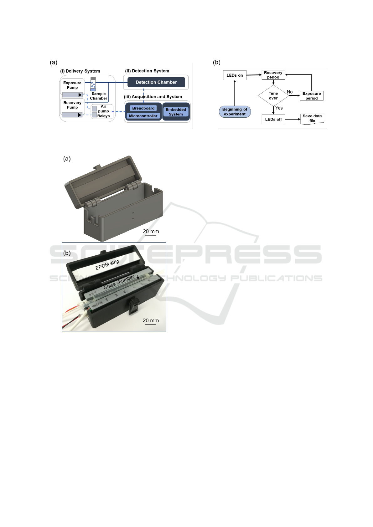
Figure 1: (a) Schematic of E-nose V3, composed by (i) Delivery system, (ii) Detection system, and (iii) Acquisition and

control system. (b) Flow of instructions given by the embedded system.

Figure 2: (a) 3D drawing of the external detection cham-

ber. (b) Printed external detection chamber, enclosing the

printed internal structure and respective connections. Lid is

open for illustration purpose.

monomer) rubber strip of the lid and the ﬁlms support.

This compression is enough to close the chamber her-

metically, for the pressures being applied in the sys-

tem. Besides, it also increases the sensor robustness

and isolates the light sensors from ambient light.

2.2.2 Internal Structure

The internal structure (see 3D drawings in Figure

3) serve as support to the PCBs, the polarizing ﬁl-

ters and the sensing ﬁlms support. It has two slots

to insert two PCBs: one that has an emission cir-

cuit with LEDs, and other that has a detection circuit

based on photodiodes. These PCBs are symmetrically

aligned in front of each other. As such, each LED

is placed exactly in front of its corresponding photo-

diode. Crossed polarizers are placed in between the

PCBs, ﬁltrating the light that is not polarized by the

sensing probes. Moreover, the light guiders prevent

interference of the light from other neighbor LEDs on

the results of each individual LED/photodiode pair.

Figure 3(e) is a picture of the fully assembled internal

structure.

Emission Circuit

The emission circuit is composed by six LEDs,

wired in parallel with the voltage source. It is a basic

LED circuit where the current is, theoretically, evenly

distributed through all the LEDs (i.e. all LEDs emit

light with equal intensity). Also, a transistor in the

common ground line acts as a switch to control LEDs.

The LEDs circuit schematic can be found in Fig-

ure 4.

Detection Circuit

Photodiodes are one of the most popular sensor

types for light-based measurements. In the present

case, the analyte detection relies on photodiodes for

precise light intensity measurement. The photodiodes

circuit schematics can be found in Figure 5.

Photodiodes generate a current proportional to the

photons that strike their active area. This current

needs to be converted into voltage, since the micro-

controller (Arduino Due) analog input pins read volt-

age variations, and not current variations. Therefore,

a circuit using a current-to-voltage converter (in this

case a transimpedance ampliﬁer) was implemented.

Here, there is a need to point out the importance of

DIV

(Figure 5) voltage. The value of V

DIV

is estab-

lished as a compromise between the output voltage

window and the reverse polarization of the photodi-

odes. The maximum output voltage is deﬁned di-

rectly by V

DIV

through the opamp (Operational Am-

pliﬁer) positive input, and the minimum is 0V, being

BIODEVICES 2019 - 12th International Conference on Biomedical Electronics and Devices

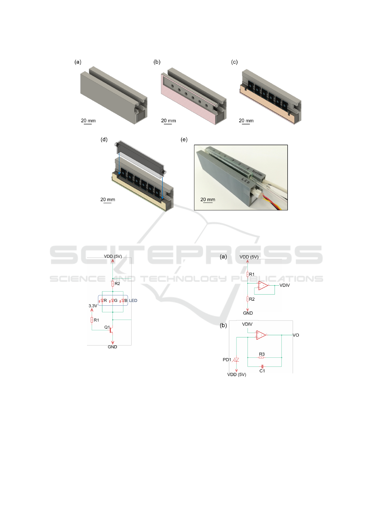
Figure 3: Main internal structure (light grey) and sensing ﬁlms support (dark grey). The sensing ﬁlms support is removable to

ease the sensing ﬁlms placement. (a) 3D drawing of the symmetrical internal structure. (b) Cross-section revealing one of the

PCBs slot and respective light-guiders for the six LED/photodiode pairs. (c) Middle cross-section revealing the sensing ﬁlms.

(d) Middle cross-section revealing how the glass chamber ﬁts in the sensing ﬁlms support. (e) Assembled internal structure

with respective components and connections.

Figure 4: Schematic of the LED´s circuit designed using

Eagle software. Only one LED is represented for illustra-

tion purposes.

the lowest value read by the arduino analog inputs

(3.3 - 0V range). On the other hand, photodiode´s

reverse polarization voltage is the result of V

minus

the opamp negative input voltage (or V

DIV

, since both

inputs share the same voltage). Increasing V

DIV

will

increase the output window but negatively impact the

performance of the photodiodes, as they beneﬁt from

higher polarization voltages (become more sensitive

to light). Opposite behaviour occurs if V

DIV

is de-

creased.

Figure 5: Schematic of photodiode´s circuit designed using

the software Eagle. (a) Generic voltage divider to gener-

ate V

DIV

. (b) Schematic of photodiode´s reverse polarizing

circuit. One replica per photodiode.

A viable way to also control the system sensitiv-

ity to light is by resizing the resistor in the negative

feedback loop, according to Equation 1 (Ohm Law).

DROP

is the voltage drop at the output, I

the cur-

rent generated by the photodiode (PD) and R the re-

An Optimized E-nose for Efﬁcient Volatile Sensing and Discrimination

sistor value. The resizing of this resistor can be seen

as an adjusting scale for the output signal, avoiding

signal saturation.

DROP

= R.I

(1)

To conﬁrm that the detection circuit is properly

working without signal loss, either through signal sat-

uration or insufﬁcient sensitivity of the photodiodes

to the lowest amounts of photons, one more test was

performed.

A new setup (Figure 6) was assembled, including

polarizing ﬁlters, and where a single LED/photodiode

pair had the ability to rotate over the other. The ex-

periment aimed to conﬁrm that the photodiodes were

sensitive enough to detect small light variations, spe-

cially close to the darkest point (i.e. when polariz-

ers are crossed at 90°) corresponding to the maximum

output voltage.

2.3 Acquisition and Control System

The instructions to control the device are given by an

embedded system (Raspberry Pi 3 Model B) and exe-

cuted by a microcontroller (Arduino Due). When the

experiment begins, the LEDs are turned on, and the

pumps work alternately while the photodiodes receive

the signal and the microcontroler acquires them at a

90Hz sampling rate. At the end of the experiment, the

LEDs are turned off and data is stored in a text ﬁle for

later analysis (see Figure 1(b)). In terms of software,

the latest version of the open access language Python

(Python 3.6) was used with Pymata library, that al-

lows the communication between the embedded sys-

tem and the microcontroller.

3 CLASSIFICATION TOOLS

Together with the optimization of the device, anal-

ysis tools based on Python libraries (SciPy, sklearn

and novainstrumentation) were also developed. A

machine learning algorithm was trained with a set

of selected features in order to distinguish 11 VOCs.

In these tests, a single sensing ﬁlm composition was

used.

Before extracting the features of the signal, the

signal was ﬁltered using the median ﬁlter from SciPy

library, kernel size equal to 11, to remove inductive

noise caused mainly by the activation of the pumps.

Then, the signal was ﬁltered with smooth function

from the novainstrumentation library. The E-nose

records information that indicates when the recovery

or the exposure pumps are working. This information

was used to split the signal and obtain the individual

cycles (a cycle corresponds to exposure to gas sam-

ple followed by a recovery period, in which air re-

stores the radial conﬁguration of the LC-IL droplets,

see Figure 7. Full phenomenon is described by (Hus-

sain et al., 2017).). Every time there is an indication

that the exposure pump is on, a cycle begins and a cut

in the signal is made (Figure 8(a)).

After splitting the signal in individual cycles,

those were normalised by Equation 2.

signal

normalized

∑

value

− min(signal)

max(signal) − min(signal)

(2)

A time domain analysis was performed, combin-

ing two types of features: morphological features and

parameters of curve ﬁtting models.

A typical output signal, regarding an individual

cycle, starts to rise when the sensors are being ex-

posed to VOCs, until a maximum is reached which

corresponds to the darkest state. On the other hand,

the output signal decreases as the VOCs leave the

chamber, restoring the radial conﬁguration of the

droplets and corresponding to the brightest state. This

leads to a typical shape in the derivatives. Figure 8(b)

represents a single cycle and its respective derivatives.

The ﬁrst derivative has two prominent peaks, with

their position corresponding to the inﬂection points

in the rise (positive peak) and the decrease (nega-

tive peak) of the signal. The second derivative has

four prominent peaks; two positives when the signal

is concave up and two negatives where it is concave

down. The relative position of these peaks in relation

to the beginning of the cycle, as well at its amplitudes,

correspond to the ﬁrst thirteen extracted features.

A suggestion made by R. Dutta and col-

leagues (Dutta and Dutta, 2006) was followed. Skew-

ness and kurtosis which are measures of the asymme-

try of the probability distribution of a random vari-

able around its mean were extracted. Although the

signal is not a probability density function, extracting

these features helped increase the accuracy of their

electronic nose classiﬁer. Hence, they were included

to see if could also be ﬁtted for the current problem.

For the ﬁtting model, the function considered was

proposed by Holmberg, M. et al. (Equation 3) where

corresponds to signal amplitude, θ

to the rising

slope, θ

to the position where the signal reaches half

the rise, θ

to the descent slope and θ

to position

where the signal reaches half of the descend (Holm-

berg et al., 1998). This model is based on the logis-

tic function (Equation 4). The logistic function de-

scribes something that initially grows and that even-

tually starts to saturate and converge to a maximum

value (in this case, total darkness, that occur when the

droplets’ conﬁguration becomes isotropic). In Equa-

BIODEVICES 2019 - 12th International Conference on Biomedical Electronics and Devices

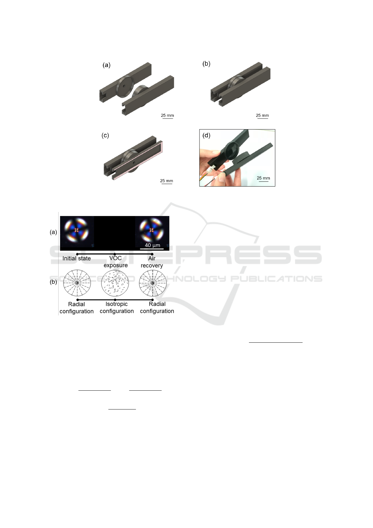
Figure 6: 3D printed structures designed to verify the detection circuit. (a) Separated pieces revealing the interior of the round

chamber. (b) When together they create an isolated dark chamber, where the center point is the light-guider of the respective

LED/photodiode pair. (c) Cross-section revealing the PCB slot. (d) Printed and assembled structure as used in the test.

Figure 7: (a) Polarized Optical Microscopy image of a

droplet when it interacts with a VOC. (b) Illustration of con-

ﬁguration changes when the VOC interacts with a droplet.

Adapted from (Hussain et al., 2017).

tion 4, parameter a corresponds to that maximum

value, b is the steepness of the curve and c indicates

when in time the curve reaches its mid point.

f (x) = θ

1 + e

.(θ

−x)



1 −

1 + e

.(θ

−x)



(3)

f (x) =

1 + e

b.(c−x)

(4)

The wrapper method Recursive Feature Elimina-

tion with Cross Validation (RFECV) was used for

feature selection. This algorithm recursively elimi-

nates features and in each iteration trains a classiﬁer

to ascertain the effect of the removed feature. It stops

when a good classiﬁcation score is obtained. It then

ranks feature performance as 1 if the remaining subset

of features gave a good classiﬁcation result. A. Jovic

et al. stated that linear Support Vector Machines were

feasible to use with wrapper methods (Jovic et al.,

2015). Therefore, it was the learning model used.

Stratiﬁed 10-fold cross-validation was used to obtain

a classiﬁcation score. In which the dataset is ran-

domly divided in ten subsets, avoiding unbalanced set

by mantaining class percentage, and using one tenth

of the set as validation set and the rest as training set.

Then the process is repeated ten times and the result

is the average of the accuracies obtained.

Accuracy, given by Equation 5, was chosen as the

scoring method, since it provides a measure of global

performance.

Accuracy =

T P + T N

T P + T N + FP + FN

(5)

It gives the number of correctly classiﬁed exam-

ples: the sum of True Positives (TP) and True Nega-

tives (TN) divided by the total number of examples

(TP, TN, False Positives (FP) and False Negatives

(FN)).

Finally, a Support Vector Machine classiﬁer was

chosen as the classiﬁcation model. The standard

SVM, illustrated in Figure 9, is a binary classiﬁer. It

ﬁnds a hyperplane that best separates the two classes

and creates a decision boundary. The examples of the

classes that are closer to the hyperplane are called the

support vectors. The hyperplane can be described by

the set of points that satisfy w

x = 0, w being the

vector perpendicular to the hyperplane. The points

An Optimized E-nose for Efﬁcient Volatile Sensing and Discrimination

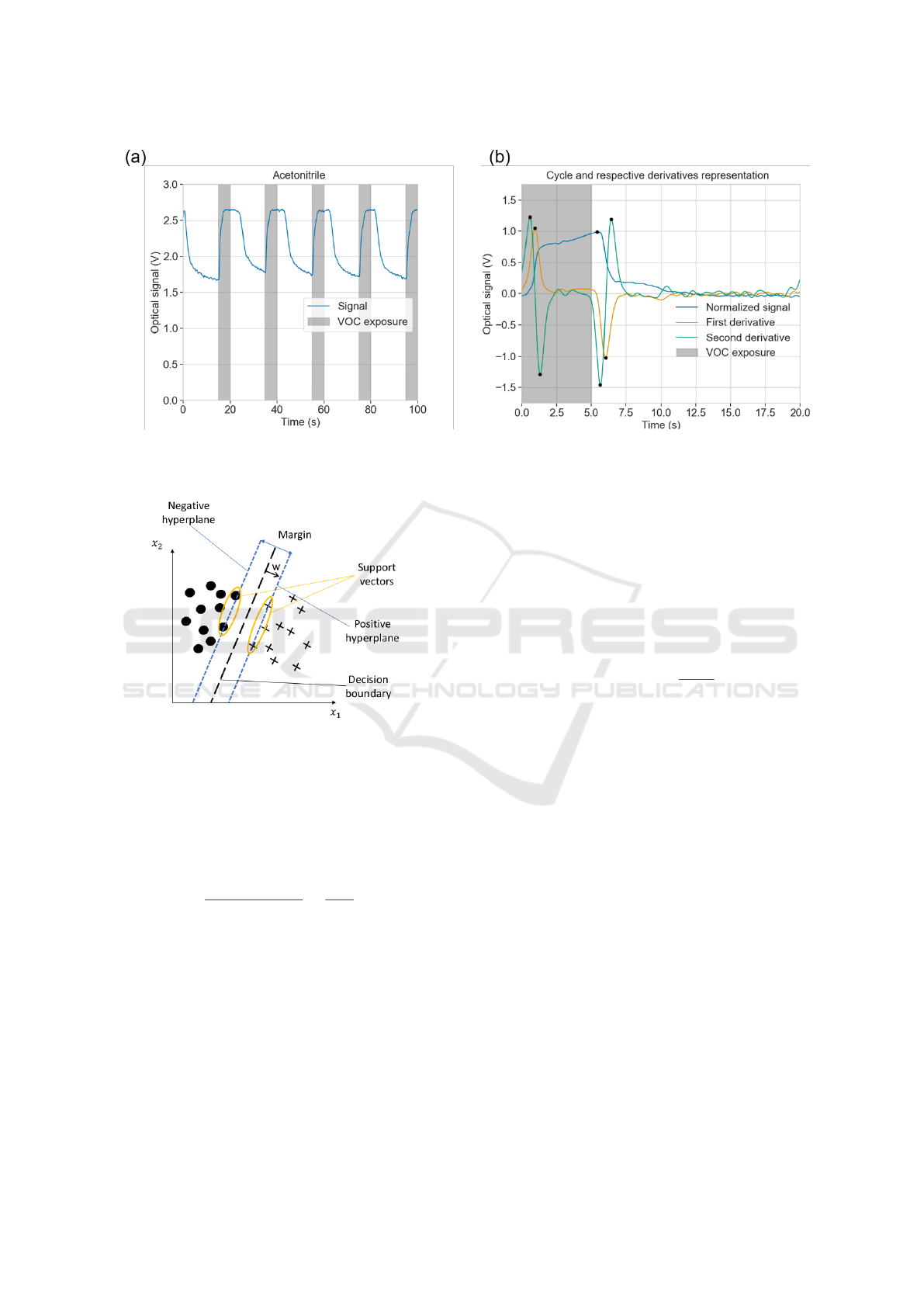
Figure 8: (a) Representation of some cycles with their exposure and recovery times. (b) Example of an individual cycle and

its ﬁrst and second derivatives. Black dots mark the peaks of interest and the darkened part of the plot correspond to the

exposure time.

Figure 9: Schematic representation of Support Vector Ma-

chines. Adapted from (Sebastian, 2015).

that satisfy w

+ w

pos

= 1 form the positive hyper-

plane, and the ones that satisfy w

+ w

neg

= −1

form the negative hyperplane. By subtracting those

expressions and normalizing by the length of the vec-

tor w, Equation 6 is obtained.

pos

− x

neg

)

||w||

(6)

The left term of Equation 6 is the distance between

hyperplanes, the objective is to maximize it.

The performance of the SVM classiﬁer depends

on the kernel, the kernel parameter γ (if kernel is non-

linear) and the parameter C.

The variable C inﬂuences the number of support

vectors used by the model, a larger C means a higher

cost for misclassiﬁcation (Sebastian, 2015).

The kernel is used to transform the original fea-

tures and project them onto a higher dimensional

space via a mapping function (Sebastian, 2015). The

kernels available in the scikit-learn library were:

polynomial kernel, radial basis function kernel, and

sigmoid kernel.

The radial basis function kernel, the one used in

this work, is deﬁned by Equation 7. The parameter γ

inﬂuences the reach of the training examples, a higher

γ makes the boundaries closer to the examples. By

default, its value is 1/nr

samples

K(x, x

) = e



−

||x−x

2σ



= e

(

−γ||x−x

)

(7)

Parameters C and γ should be tuned together. For

that, is possible to use GridSearchCV from scikit-

learn library that performs a grid search with cross

validation to choose the best parameters. This func-

tion was used with: values 0.1, 1, 10 and 100 for C;

values 0.01, 0.8, 1 and 10 for γ; and the kernels avail-

able, already mentioned. Other parameters from the

SVC scikit-learn library used the default values given.

4 RESULTS

4.1 Features of E-nose V3

E-nose V3 is an optimized version of E-nose V0, the

ﬁrst prototype. The system was improved, having a

faster and cheaper data acquisition system composed

by an Arduino microcontroller and a Raspberry Pi

(under 100 euros) as opposed to the previous system

composed by a computer and a NI myDAQ (above

600 euros). Now it possess a single interface making

BIODEVICES 2019 - 12th International Conference on Biomedical Electronics and Devices

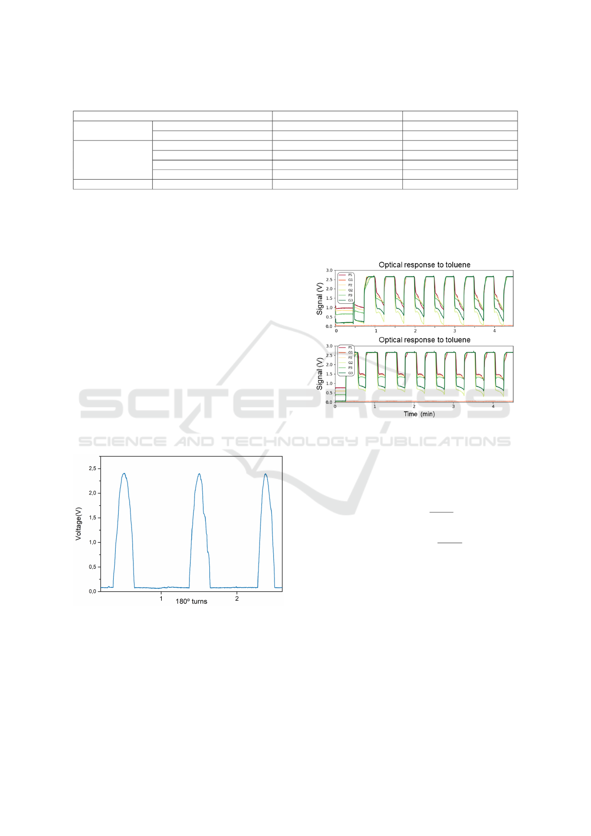
Table 1: Comparative table of different e-nose versions.

E-nose Version First version (P

adua et al., 2018b) Latest version (present work)

Transduction system

Sampling rate (Hz) 10 90

Data acquisition elements NI myDAQ + Computer Arduino Due + Raspberry Pi3

Detection chamber

Detection sensors Photoresistors Photodiodes

Array capacity (nr sensors)

4 6

Stability and scaling (scale 1-5)* 1 4

Chamber volume 2L 28mL

Delivery system Analysis frequency 0.37 cycles/min 3 cycles/min

* Stability and scaling scale:

1: Open and close the chamber was not practical. Chamber with ﬂow losses.

2: Robust and more easy-to-use chamber. Difﬁcult to change sensing ﬁlms between experiments. Flow losses veriﬁed.

3: Easy to change sensing ﬁlms. Hermetic. PCBs with through-hole technology. components.

4: Easy to change sensing ﬁlms. Hermetic.. PCBs with surface-mount technology components. Has slots to insert the PCBs and support for sensing

ﬁlms. Has light guiders for LEDs.

it more user-friendly (P

adua et al., 2018a). Regarding

the detection chamber, the number of sensors was in-

creased and the chamber became more robust, stable

and hermetic. Moreover, improvements in the deliv-

ery system allowed a 10 times faster analysis, com-

paring to the initial prototype.

Regarding the delivery system, pumps ﬂow rate

is 3 L/min, the ﬂow rate at chamber entrance is 1.8

L/min for the exposure circuit, and 2.5 L/min for the

recovery circuit. Table 1 summarizes the main differ-

ences between E-nose versions.

Considering the implementation of a new detector

system, the results for the validation of the photodi-

odes are represented in Figure 10. It demonstrates

that the photodiodes are suitable for the application

and that no signal is lost at any given light intensity.

Figure 10: Proof of concept of the photodiodes sensitivity.

The experiment consisted in the signal acquisition during

three 180 degree turns. The absence of a saturation line at

the maximum values approves the detection system.

Signals were acquired (Figure 11) to test the new

version of the E-nose. A preliminary experiment was

made to measure signal to noise ratio. Five sens-

ing ﬁlms were sequentially exposed to two different

VOCs (acetone and toluene), the remaining position

Figure 11: Signals acquired to test the new E-nose version.

Position G1 corresponds to the control measurement.

of the array was used as a control measurement.

The signal to noise ratio (SNR) was calculated by

Equation 8. The result was approximately 50 dB.

SNR

= 10log



signal

noise



= 20log



signal

noise



(8)

4.2 Classiﬁcation Results

Three sensing gels, with the exact same composition,

were exposed to a sequence of 11 VOCs (hexane, hep-

tane, toluene, chloroform, dichloromethane, acetoni-

trile, acetone, diethyl ether, ethyl acetate, ethanol and

methanol) in cycles of 5 seconds of exposure and 15

seconds of recovery. 15 mL of VOC were placed in

the sample chamber and heated at 37°C durign 15

minutes before beggining the experiment to ensure

headspace saturation. Each sample interacted with

the sensors in a total of 15 minutes. The remaining

positions of the electronic nose were used as control

An Optimized E-nose for Efﬁcient Volatile Sensing and Discrimination

measurements. After the sequence was completed,

sensing gels were stored. Two months later, the same

procedure was repeated with the same sensing gels.

The ﬁrst cycles of each volatile (the ﬁrst 5 for the ﬁrst

time the gels were exposed and the ﬁrst 6 for the sec-

ond time) were not considered due to the presence of

noise, caused by the opening of the valve that allows

VOC intake. This resulted in a total of approximately

2600 cycles for analysis (236 cycles per VOC).

The features were extracted, however, the curve

ﬁtting algorithm was not able to converge into a solu-

tion for the parameters of the approach of the article

(Equation 3). In order to ﬁt a model to the signal,

it was necessary to simplify the approach. The solu-

tion was to divide the signal in two parts (from cycle

beginning until its maximum and from the maximum

until its end) and apply the logistic function (Equation

4) to each part of the signal (Figure 12).

Figure 12: Estimated curves for (a), the ﬁrst part of the cy-

cle and for (b), the second part. The red point marks the

coordinates where the signal bisects with the value of half

the rise/descend.

After obtaining a set of features, RFECV algo-

rithm used a quarter of the data and the rest remained

untouched for validation purposes. The rank of the

features is shown in Table 2. Features ranked as 1 are

the ones with best performance, and therefore were

the ones selected.

When tuning the classiﬁer parameters, the best

performance was obtained with the radial basis func-

tion kernel and parameters C: 100 and γ : 0.1.

Finally, to validate the classiﬁer with unseen data,

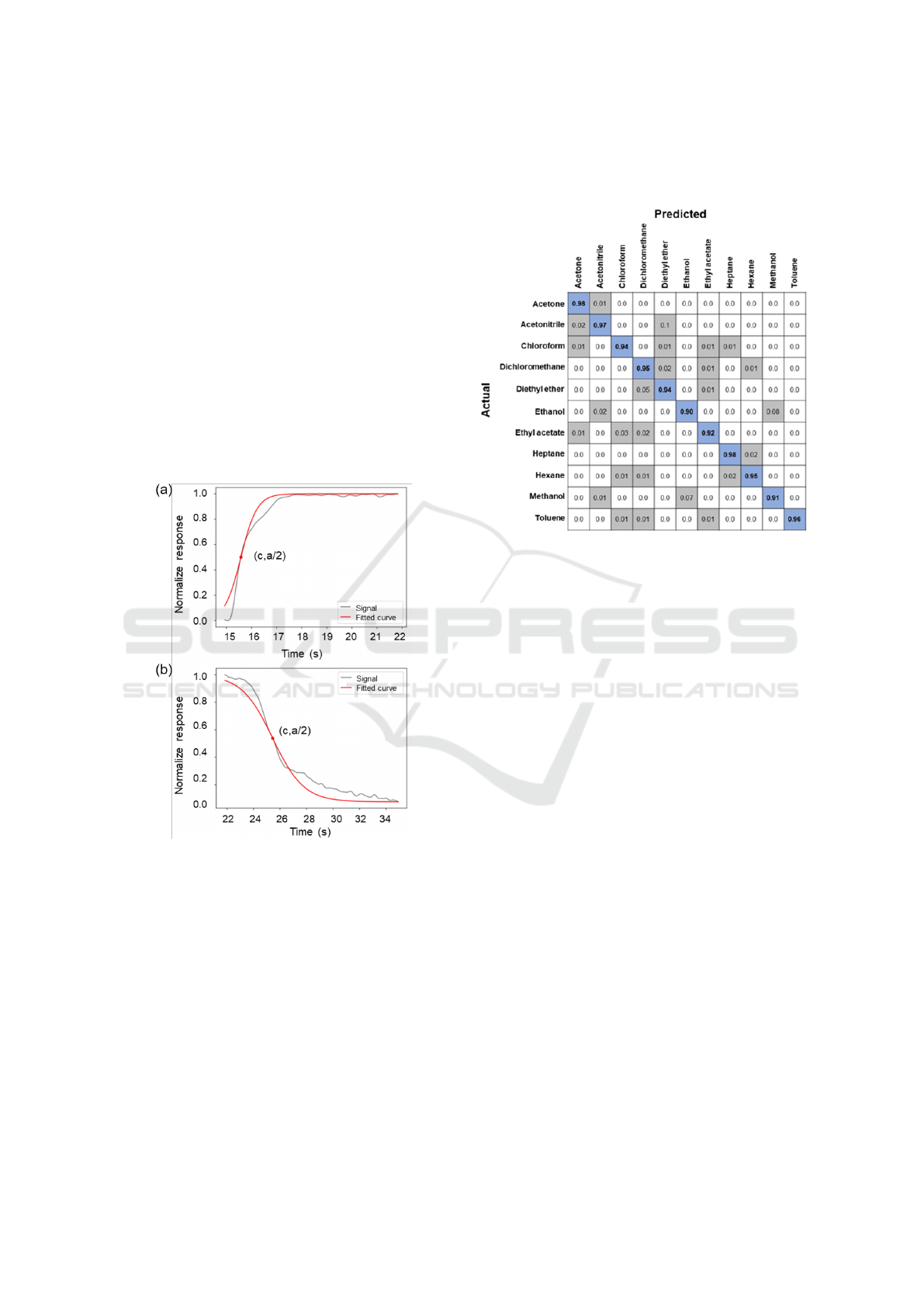
the validation set was used. The classiﬁer managed

to obtain a global accuracy of 94.6% with a standard

deviation of 0.9%. Figure 13 shows the correspondent

normalized confusion matrix.

Figure 13: Confusion matrix obtained for the classiﬁcation

of the 11 VOCs. Accuracy of 94.6% (± 0.9%).

5 CONCLUSION AND FUTURE

WORK

E-nose V3 is a tailor-made device using as gas sen-

sors an innovative class of biomaterials which opti-

cal properties vary in the presence of VOCs (Hus-

sain et al., 2017). This new optimized device, to-

gether with the appropriate use of signal processing

tools, allowed the accurate classiﬁcation of 11 VOCs

from different chemical classes using sensing ﬁlms

with the exact same composition. The results show

that our sensor possess advantages over other types

of sensors such as MOS-sensors or conducting poly-

mer sensors, as these normally have limited selectiv-

ity towards VOC classes. In addition, our materials

and sensing device operate at ambient conditions as

opposed to MOS (300°C)(Wilson, 2012). In addition,

used sensing materials are biodegradable and reusable

with the potential to recycle its individual compo-

nents, having a lower carbon footprint.

The detection chamber is hand-size and hermetic

for the pressures being applied. Its low volume allows

the use of short cycle periods, and consequently a fast

analysis. The advantages of using photodiodes is that

they are more sensible and have a quicker response

time than photoresistors.

The transduction system based on Arduino and

Raspberry Pi constitute a low-cost and independent

BIODEVICES 2019 - 12th International Conference on Biomedical Electronics and Devices

Table 2: Ranking of the selected features by RFECV with 10-fold cross validation.

Number Description 10-fold validation score

1 Time to reach the maximum value of the cycle 7

2 Time to reach the maximum of the ﬁrst derivative of the signal 4

3 Time to reach the minimum of the ﬁrst derivative of the signal 1

4 Maximum value of the ﬁrst derivative of the signal 3

5 Minimum value of the ﬁrst derivative of the signal 2

6 Time to reach the maximum of the ﬁrst half of the second derivative of the signal 1

7 Time to reach the minimum of the ﬁrst half of the second derivative of the signal 10

8 Maximum value of the ﬁrst half of the second derivative of the signal 1

9 Minimum value of the ﬁrst half of the second derivative of the signal 1

10 Time to reach the maximum of the second half of the second derivative of the signal 11

11 Time to reach the minimum of the second half of the second derivative of the signal 9

12 Maximum value of the second half of the second derivative of the signal 1

13 Minimum value of the second half of the second derivative of the signal 1

14 Area under the signal 1

15 Skewness 1

16 Kurtosis 1

17 Parameter a from the ﬁrst half of the signal 13

18 Parameter b from the ﬁrst half of the signal 1

19 Parameter c from the ﬁrst half of the signal 1

20 Error associated with the ﬁt from the ﬁrst half of the signal 5

21 Parameter a from the second half of the signal 12

22 Parameter b from the second half of the signal 1

23 Parameter c from the second half of the signal 6

24 Error associated with the ﬁt from the second half of the signal 8

unit. The sampling rate of 90 Hz was enough to guar-

antee informative signal acquisition.

After data collection, two different feature extrac-

tion methods were used: features extraction from the

original response curves and curve ﬁtting parameters.

The most informative features extracted from the sig-

nals were identiﬁed and reported in bold in Table 2.

Applying those features, the accuracy rate for SVM

was 94.6% ± 0.9%. Future work should include com-

parison of these results with other machine learning

classiﬁcation techniques.

The assembled system was able to distinguish the

11 tested VOCs. Although the identiﬁcation of the

VOCs was not made in real time, a step towards mak-

ing this E-nose a device that is able to make automatic

classiﬁcation was taken.

The E-nose V3 device is robust and user-friendly.

We are aware that there is still room for improvement.

For example, in the future the detection system could

beneﬁt from the use of variable resistors, or multiple

resistors per photodiode, enabling auto scaling or sim-

ply by easing the actual scaling where multiple PCBs

assembled with different resistor values, are chosen to

best suit the sensing probes in use based on the out-

put voltage. Also, a longer array of LED/photodiodes

pairs would allow for a wider combination of different

sensing probes, or a larger number of replicas, which

in both cases have a positive impact in the VOCs pre-

diction algorithm.

Using the optimized e-nose version, the necessary

studies to evaluate more complex scenarios are pos-

sible, such as testing concentration limits, the effects

of room conditions in the material and classiﬁcation

of complex samples where many different VOCs are

mixed together.

ACKNOWLEDGEMENTS

This project has received funding from the European

Research Council (ERC) under the EU Horizon 2020

research and innovation programme (grant agree-

ment No. SCENT-ERC-2014-STG-639123). This

work was supported by the Applied Molecular Bio-

sciences Unit-UCIBIO which is ﬁnanced by national

funds from FCT/MCTES (UID/Multi/04378/2013)

and co-ﬁnanced by ERDF under the PT2020 Partner-

ship Agreement (POCI-01-0145-FEDER-007728).

The authors thank FCT/MEC for the research fellow-

ship PD/BD/105752/2014 for A.P.

REFERENCES

Arshak, K., Moore, E., Lyons, G., Harris, J., and Clifford,

S. (2004). A review of gas sensors employed in elec-

tronic nose applications. Sensor Review, 24(2):181–

198.

Barbosa, A. J., Oliveira, A. R., and Roque, A. C. A. (2018).

An Optimized E-nose for Efﬁcient Volatile Sensing and Discrimination

Protein- and peptide-based biosensors in artiﬁcial ol-

faction. Trends in Biotechnology, 36:1244–1258.

Dutta, R. and Dutta, R. (2006). Intelligent Bayes Classi-

ﬁer (IBC) for ENT infection classiﬁcation in hospital

environment. BioMedical Engineering Online, 5.

Ghasemi-Varnamkhasti, M., Mohtasebi, S. S., Siadat, M.,

Ahmadi, H., and Razavi, S. H. (2015). Research pa-

per: From simple classiﬁcation methods to machine

learning for the binary discrimination of beers using

electronic nose data. Engineering in Agriculture, En-

vironment and Food, 8:44 – 51.

He, Q., Yan, J., Shen, Y., Bi, Y., Ye, G., Tian, F., and

Wang, Z. (2012). Classiﬁcation of Electronic Nose

Data in Wound Infection Detection Based on PSO-

SVM Combined with Wavelet Transform. Intelligent

Automation and Soft Computing, 18(7):967–979.

Holmberg, M., Gustafsson, F., H

ornsten, E. G., Winquist,

F., Nilsson, L. E., Ljung, L., and Lundstr

om, I.

(1998). Bacteria classiﬁcation based on feature ex-

traction from sensor data. Biotechnology Techniques,

12(4):319–324.

Hussain, A., Semeano, A. T. S., Palma, S. I. C. J., Pina,

A. S., Almeida, J., Medrado, B. F., P

adua, A. C.

C. S., Carvalho, A. L., Dion

ısio, M., Li, R. W. C.,

Gamboa, H., Ulijn, R. V., Gruber, J., and Roque,

A. C. A. (2017). Tunable gas sensing gels by co-

operative assembly. Advanced Functional Materials,

1700803:1–9. ¡p¿n/a¡/p¿.

Jovic, A., Brkic, K., and Bogunovic, N. (2015). A re-

view of feature selection methods with applications.

In 2015 38th International Convention on Information

and Communication Technology, Electronics and Mi-

croelectronics (MIPRO), pages 1200–1205.

Ordukaya, E. and Karlik, B. (2017). Quality control of olive

oils using machine learning and electronic nose. Jour-

nal of Food Quality, Vol 2017 (2017).

adua, A. C., Os

orio, D., Rodrigues, J., Santos, G., Porteira,

A., Palma, S., Roque, A., and Gamboa, H. (2018a).

Scalable and easy-to-use system architecture for elec-

tronic noses. In Proceedings of the 11th International

Joint Conference on Biomedical Engineering Systems

and Technologies, pages 179–186.

adua, A. C., Palma, S., Gruber, J., Gamboa, H., and

Roque, A. C. A. (2018b). Design and evolution of

an opto-electronic device for vocs detection. Pro-

ceedings of the 11th International Joint Conference on

Biomedical Engineering Systems and Technologies,

pages 48–55.

ock, F., Barsan, N., and Weimar, U. (2008). Electronic

nose: Current status and future trends. Chemical Re-

views, 108(2):705 – 725.

Scott, S. M., James, D., and Ali, Z. (2007). Data analy-

sis for electronic nose systems. Microchimica Acta,

156(3/4):183 – 207.

Sebastian, R. (2015). Python Machine Learning. Packt Pub-

lishing Ltd.

Uc¸ar, A. and

Ozalp, R. (2017). Efﬁcient android elec-

tronic nose design for recognition and perception of

fruit odors using kernel extreme learning machines.

Chemometrics and Intelligent Laboratory Systems,

166:69 – 80.

Wasilewski, T., Ge¸bicki, J., and Kamysz, W. (2017).

Bioelectronic nose: Current status and perspectives.

Biosensors and Bioelectronics, 87:480–494.

Wilson, A. D. (2012). Review of electronic-nose tech-

nologies and algorithms to detect hazardous chemi-

cals in the environment. Procedia Technology, 1(First

World Conference on Innovation and Computer Sci-

ences (INSODE 2011)):453 – 463.

Xu, L., He, J., Duan, S., Wu, X., and Wang, Q. (2016).

Comparison of machine learning algorithms for con-

centration detection and prediction of formaldehyde

based on electronic nose. Sensor Review, 36(2):207.

Yan, J., Xiuzhen, G., Shukai, D., Pengfei, J., Lidan, W.,

Chao, P., and Songlin, Z. (2015). Electronic nose fea-

ture extraction methods: A review. Sensors, Vol 15,

Iss 11, Pp 27804-27831 (2015), (11):27804.

BIODEVICES 2019 - 12th International Conference on Biomedical Electronics and Devices