Learning Task-speciﬁc Activation Functions using Genetic Programming

Mina Basirat and Peter M. Roth

Institute of Computer Graphics and Vision, Graz University of Technology, Graz, Austria

Keywords:

Deep Neural Networks, Activation Functions, Genetic Programming.

Abstract:

Deep Neural Networks have been shown to be beneﬁcial for a variety of tasks, in particular allowing for end-to-

end learning and reducing the requirement for manual design decisions. However, still many parameters have

to be chosen manually in advance, also raising the need to optimize them. One important, but often ignored

parameter is the selection of a proper activation function. In this paper, we tackle this problem by learning task-

speciﬁc activation functions by using ideas from genetic programming. We propose to construct piece-wise

activation functions (for the negative and the positive part) and introduce new genetic operators to combine

functions in a more efﬁcient way. The experimental results for multi-class classiﬁcation demonstrate that for

different tasks speciﬁc activation functions are learned, also outperforming widely used generic baselines.

1 INTRODUCTION

Deep Neural Networks (DNNs) (Goodfellow et al.,

2016; LeCun et al., 2015) have recently become po-

pular and are now successfully applied for a wide

range of applications. However, since increasingly

more complex and deeper networks are of interest,

strategies are required to make neural network trai-

ning efﬁcient and stable. While initialization (e.g.,

(Sutskever et al., 2013; Mishkin and Matas, 2017))

and normalization techniques (e.g., (Laurent et al.,

2016)) are well studied, a relevant and important fac-

tor is often neglected: the role of activation functions

(AF).

This is illustrated Figure 1, where we show the

results of a simple experiment on a 2D dataset repre-

senting the XOR-problem. In particular, we trained

a simple neural network with only one hidden layer

consisting of only one neuron. It can be seen from

Figure 1a that using a Rectiﬁed Linear Unit (ReLU)

as Activation Function (AF), even this simple pro-

blem cannot be solved. In contrast, as shown in Fi-

gure 1b, using a more complex activation function

such as obtained by our approach we get a signiﬁ-

cantly better result.

Even though recent work demonstrated that AFs

are of high relevance (Klambauer et al., 2017; Ra-

machandran et al., 2018; Clevert et al., 2016; Elf-

wing et al., 2018; Glorot et al., 2011; Gulcehre

et al., 2016)), due to its simplicity and reliability most

deep learning approaches use Rectiﬁed Linear Units

(a) ReLU.

(b) Our approach.

Figure 1: Importance of activation functions: Using ReLU

even a simple problem like XOR-problem cannot be solved,

whereas our approach yields a meaningful solution.

(ReLU) (Nair and Hinton, 2010).

Due to their universal approximation proper-

ties, the research in this ﬁeld was concentrated on

squashing functions such as Sigmoid and Tanh (Hor-

nik, 1991). However, training DNNs using such

functions suffers from the vanishing gradient problem

(Hochreiter, 1998). To overcome this problem, vari-

ous non-squashing functions were introduced, where

the most notable one is (ReLU). In particular, as the

derivative of positive inputs in ReLU is one, the gra-

dient cannot vanish. In contrast, as all negative values

are mapped to zero, there is no information ﬂow in

DNNs for negative values, which is known as dying

ReLU.

To deal with this problem, various generalizati-

ons of ReLU such Leaky ReLU (Maas et al., 2013)

have been proposed. Similarly, Exponential Linear

Units (ELU) (Clevert et al., 2016) do not only elimi-

Basirat, M. and Roth, P.

Learning Task-speciﬁc Activation Functions using Genetic Programming.

DOI: 10.5220/0007408205330540

In Proceedings of the 14th International Joint Conference on Computer Vision, Imaging and Computer Graphics Theory and Applications (VISIGRAPP 2019), pages 533-540

ISBN: 978-989-758-354-4

533

nate the bias shift in the succeeding layers, but also

push the mean activation value towards zero by re-

turning a bounded exponential value for negative in-

puts. Although showing competitive results, ELU is

not backed by a very strong theory. A theoretically

proven extension, Scaled Exponentiation Linear Uni-

tes (SeLU) (Klambauer et al., 2017), makes DNN le-

arning more robust. In fact, it is shown that the pro-

posed self-normalizing network converges towards a

normal distribution with zero mean and unit variance.

Another direction was pursued in (Ramachandran

et al., 2018), ﬁnally introducing Swish. Different se-

arch spaces are created by varying the number of core

units used to construct the AF. In addition, an RNN is

trained to search the state space for a novel AF. The

proposed approach shows competitive results for both

shallow and deep neural networks, however, Swish

was not found by the approach but was already inclu-

ded in the initial set of candidate solutions. Recently,

a theoretic justiﬁcation for the design has been given

in (Hayou et al., 2018), showing that Swish propaga-

tes information better than ReLU. Moreover, (Penning-

ton et al., 2018) showed that Swish along with ort-

hogonal initialization provides a dynamical isometry,

which allows for faster learning. Thus, existing ap-

proaches to estimate AFs are lacking theoretical foun-

dation, are based on complex theory, which is hard to

understand in the context of practical applications, or

are based on inefﬁcient search schemes, which still

require to manually set several parameters.

To overcome these problems and to avoid the need

for prior information (as in the case of Swish), we

propose an approach based on ideas of Genetic Pro-

gramming (GP) (Mitchell, 1996) to learn efﬁcient

activation functions better suited for a speciﬁc task. In

particular, building on neuro-evolutionary algorithms

(Schaffer et al., 1992), starting from simple initial

AFs, more complex functions can be estimated. In

particular, we deﬁne a set of piece-wise functions

and combine them over several iterations based on

their ability to solve a speciﬁc problem. For that pur-

pose, we deﬁne new genetic operators, namely Hy-

brid Crossover and Hybrid Mutation, allowing us to

explore the speciﬁc search space (i.e., functions and

operators) in an efﬁcient way.

To demonstrate the beneﬁts of our approach, we

apply it for image classiﬁcation problems. We show

that, compared to commonly used baselines, using the

learned AFs we can obtain better classiﬁcation results

for the CIFAR-10 and CIFAR-100 benchmark data-

sets. In addition, we demonstrate that for different

tasks different AFs are learned, better representing the

characteristics of the problems.

The remainder of the paper is structured as fol-

lows: First, in Sec. 2, we discuss the related work

in the context of GP for Neural Networks. Next,

in Sec. 3, we introduce our new neuro-evolutionary

algorithm for learning task-speciﬁc AFs. Then, in

Sec. 4, we give an experimental evaluation of our ap-

proach and discuss the ﬁndings. Finally, in Sec. 5 we

summarize and conclude our work.

2 RELATED WORK

Neuroevolution, i.e., applying evolutionary algo-

rithms (EAs) in the optimization of DNNs (Whitley,

2001), is a vital ﬁeld of research. In general, there

are two main directions. First, optimizing training pa-

rameters such as hyper-parameters (Loshchilov and

Hutter, 2016) or weights (Montana and Davis, 1989;

Igel, 2003). In the latter case, in contrast to met-

hods like gradient descent, also global optima can be

estimated. Second, evolving an optimal DNN topo-

logy, which, however, is not straightforward. There-

fore, existing approaches follow two strategies: con-

structive (Qiang et al., 2010) and destructive (Han-

cock, 1992). Constructive methods start from a sim-

ple topology and gradually increase the complexity

until an optimality criterion is satisﬁed. In contrast,

destructive approaches start from an initially complex

topology and incrementally reduce the unnecessary

structures.

Recently, co-evolution of topology and weights

(TWEANNs) has shown to be more effective and ef-

ﬁcient, where the most successful approach is NEAT

(Stanley and Miikkulainen, 2002). NEAT follows

the constructive strategy and gradually evolves a sim-

ple DNN topology towards unbounded complexity by

adding nodes and connections between them while

preserving the optimality of topology. Thus, there

have been several extensions of NEAT. For instance,

in (Miikkulainen et al., 2017) two extensions, Deep-

NEAT and CoDeepNEAT, have been proposed. In

contrast to NEAT, in DeepNEAT a node represents a

layer and consists of a table of hyper-parameters (i.e.,

number of neurons ) related to it. In CoDeepNEAT,

two populations (modules and blueprints) are initia-

lized separately, where a module is a graph and re-

presents a shallow DNN. A blueprint has also a graph

structure and consists of nodes pointing out to speciﬁc

module species. Both modules and blueprints evolve

in parallel. Finally, the modules and blueprints are

combined to build the topology of the DNN.

Similarly, (Suganuma et al., 2017) explored a

CNN architecture via Cartesian GP (CGP) for image

classiﬁcation, where also high-level functions such as

convolution or pooling operations are implemented.

VISAPP 2019 - 14th International Conference on Computer Vision Theory and Applications

534

Recently, (Liu et al., 2018) proposed a constructive

hierarchical genetic representation approach for evol-

ving DNN topologies. Initialized with small popula-

tions of primitives such as convolutional and pooling

operations at the bottom of the hierarchy, the topo-

logy gets more and more complex by adding evolved

primitives into a graph structure.

Even though there has been drawn a lot of atten-

tion to TWEANNs, evolving AFs was only of limited

interest so far. The idea closest to ours is HA-NEAT

(Hagg et al., 2017). HA-NEAT (Hagg et al., 2017)

extends NEAT to evolve AFs of neurons, topology,

and weights, resulting in a heterogeneous network. In

contrast, we ﬁx the topology and evolve piece-wise

AFs on layer level. The proposed candidate solutions

are more complicated (advanced) than those of HA-

NEAT. More importantly, the complexity of evolved

AFs is, in contrast to HA-NEAT, unbounded. Mo-

reover, we can evolve our approach also along with

topology.

3 EVOLVING PIECE-WISE

ACTIVATION FUNCTIONS

The goal of this work is to estimate non-linear AFs

better suited for speciﬁc tasks. To this end, we build

on two ideas. First, as negative and positive inputs

have a different inﬂuence on learning, we propose to

use piece-wise AFs (i.e., separately deﬁned positive

and negative parts). Second, as the search space can

be very large, we propose to build on the ideas of Ge-

netic Programming to allow for a more efﬁcient se-

arch.

3.1 Genetic Programming

Genetic Programming (GP) (e.g., (De Jong, 2006)),

can be seen a population-based meta-heuristic to

solve problems in the ﬁeld of stochastic optimization.

In particular, we are given a large set of candidate so-

lutions, referred to as population, but we do not know

how to estimate the optimal solution for the given

task. The main idea to overcome this problem is to

evolve a population towards a better solution.

The evolution typically starts from a population

consisting of randomly selected candidate solutions,

called individuals. These are described by a set of

properties (gens), which can be altered by three bio-

inspired operations: (a) selection, (b) crossover, and

lecting individuals according to their ﬁtness. In con-

trast, crossover is a stochastic operator, exchanging

information between two individuals (often called pa-

rents: mom and dad) to form a new offspring. Simi-

larly, mutation is also a stochastic operator, helping to

increase the diversity of the population by randomly

choosing one or more genes in an offspring and chan-

ging them.

Then, in an iterative process, where we refer an

iteration to as generation, each individual is evaluated

and based on their ﬁtness, we select a set of parents

solutions for breeding. Subsequently, we apply bree-

ding operators on pairs of individuals to generate new

pairs of offsprings. Eventually, we update the popula-

tion with the set of parents and bred offsprings. This

process is repeated until a pre-deﬁned number of ge-

nerations or a pre-deﬁned optimality criterion is met.

3.2 Breeding Operators

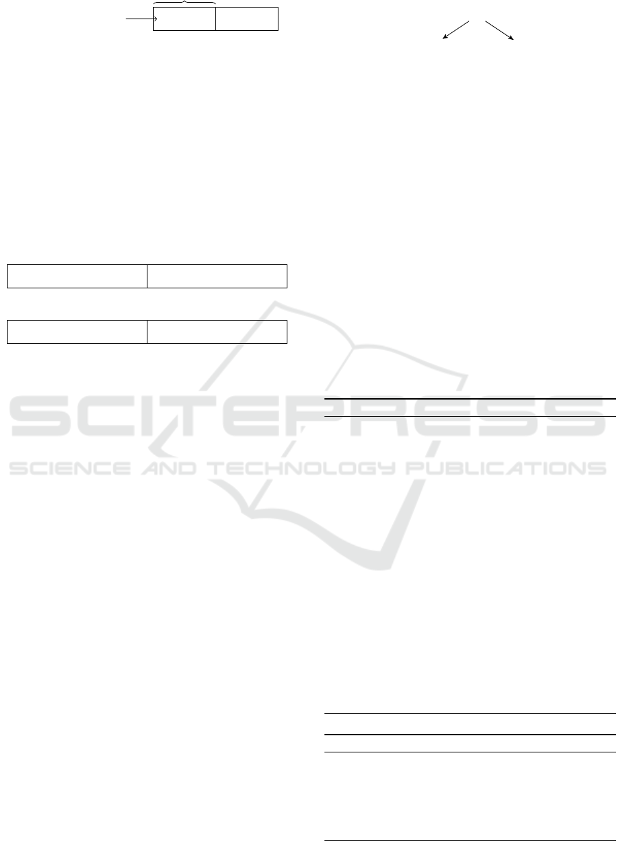
Targeting to evolve piece-wise AFs, each individual

in our population represents an AF, where a gene is

either the left or the right part of an AF (see Figure 2).

activation left

activation right

Gene

Figure 2: An individual in the population of our GP.

To evolve AFs as described above, we introduce new

operators representing our speciﬁc problem.

3.2.1 Inheritance Crossover

The Inheritance Crossover operator inherits genes

from both parents. The ﬁrst (second) offspring inher-

its its left AF from the mom (dad), and its right AF

from the dad (mom). This way, the operator resem-

bles a one-point crossover operator. However, as we

are dealing with piece-wise functions the cutoff point

is pre-determined. This is illustrated in Figure 3.

mom’s left

dad’s right

(a) Offspring 1

dad’s left

mom’s right

(b) Offspring 2

Figure 3: Inheritance Crossover.

3.2.2 Mutation Operator

The Mutation operator randomly chooses a gene and

then replaces it with a randomly selected pre-deﬁned

AF. In fact, this helps our approach to further explore

the search space for new AFs. This is illustrated in

Figure 4.

Learning Task-speciﬁc Activation Functions using Genetic Programming

535

mom’s left

Selected Activation:

ReLU

dad’s right

Selected Gene

Figure 4: Mutation operator.

3.2.3 Hybrid Crossover

To combine multiple AFs, we additionally introduce

the Hybrid Crossover operator. As for Inheritance

Crossover, the cutoff point is ﬁxed. Using a randomly

selected mathematical operator, the ﬁrst (second) off-

spring combines mom’s and dad’s (dad’s and mom’s)

negative part of the AF to form its own negative part.

Subsequently, the ﬁrst (second) offspring’s positive

part of the AF is formed via a combination of mom’s

and dad’s (dad’s and mom’s) positive part, as illustra-

ted in Figure 5.

: mom’s left : dad’s left

: mom’s right : dad’s right

(a) Offspring 1

: dad’s left : mom’s left

: dad’s right : mom’s right

(b) Offspring 2

Figure 5: Hybrid Crossover operator, where op

and op

are chosen randomly.

3.2.4 Hybrid Mutation Operator

The Hybrid Mutation operator helps our approach to

discover any possible combination of AFs. Thus, it

ﬁrst picks two random pre-deﬁned AFs and combi-

nes them with a random operator. Then it replaces a

randomly chosen gene with newly the generated AF.

3.3 Evaluating of Activation Functions

The Hybrid crossover operator generates hybrid AFs,

that we evaluate by parsing according to the following

grammar:

expression := f | (operation : expression : expression)

operation :=+ | − | × | / |min |max

f := HardSigmoid | Sigmoid | ELU | (1)

Linear | ReLU | SeLU | Softplus | . . .

where f represents the set of candidate solutions. The

list is not ﬁxed, and we can easily add additional

operations and candidate solutions f .

Example: Given an AF generated by Hybrid crosso-

ver:

(× : Softplus : ELU) .

To compute the equivalent inﬁx expression, we use

(1) and parse above AF, as shown in Figure 6:

Softplus × ELU

Softplus

ELU

Figure 6: The parse tree of Softplus × ELU.

3.4 Learning Activation Functions

After deﬁning the genetic operators and explaining

the function evolution, we can describe our appro-

ach as summarized in Algorithm 1. Initially, we ge-

nerate a population of random AFs (line 3). Next,

by using the evaluate operator (line 4) the ﬁtness of

each AF is determined according to the classiﬁca-

tion performance on an independent test set. Then,

our approach selects a set of parent AFs based on

their ﬁtness for breeding (line 7). To generate new

AFs (line 11), we ﬁrst apply the Crossover opera-

tors and then the Mutation operator as deﬁned in

Sec. 3.2. When applying the Crossover operator we

stochastically choose between Inheritance and Hybrid

as shown in Algorithm 2. Similarly, we update our

population with the set of parents and bred offsprings.

This procedure is iterated until a pre-deﬁned optima-

lity criterion is met.

Algorithm 1: GP.

1: procedure GP(population-size)

2: population ←

3: population ← INITIALIZE(population-size)

4: EVALUATE(population)

5: repeat

6: children ←

7: parents ← SELECT(population, 30%)

8: for i ≤ (population-size −|parents|)/2 do

9: increment i by one

10: hmom, dadi ∈ parents × parents

11: offsprings ← CROSSOVER(mom, dad)

12: for offspring ∈ offsprings do

13: offspring ← MUTATE(offspring)

14: EVALUATE(offsprings)

15: children ← children ∪ offsprings

16: population ← parents ∪ children

17: until termination condition

18: return population

Algorithm 2.

1: procedure CROSSOVER(mom, dad)

2: c ← toss a coin

3: if c is heads then

4: return INHERITANCE(mom, dad)

5: return HYBRID(mom, dad)

VISAPP 2019 - 14th International Conference on Computer Vision Theory and Applications

536

4 EXPERIMENTAL RESULTS

To demonstrate the beneﬁts of our approach, in

Sec. 4.3, we apply the approach for two real-world

benchmark datasets of different complexity, namely

CIFAR-10

and CIFAR-100

. This way, we are also

able to show that for different tasks different choices

of AFs are meaningful. Moreover, to demonstrate the

generality of the evolved AFs, we apply them to dif-

ferent architectures (i.e., ResNet (He et al., 2016) vs.

VGG (Simonyan and Zisserman, 2015)). In addition,

we give a baseline comparison to a random search for

learning AFs in Sec. 4.2. For all experiments, we used

the same experimental setup, which we describe in

Sec. 4.1.

4.1 Experimental Setup and

Implementation Details

Similar to (Ramachandran et al., 2018), we run our

approach on shallow architectures (i.e., ResNet20).

Then we use the learned AFs to train deeper networks

(i.e., Resnet56). Moreover, to demonstrate that the le-

arned functions are of general interest, we use them

to train classiﬁers using the VGG-16 architecture. To

this end, we used the default parameters for both ar-

chitectures. To avoid random effects, all networks

have been initialized using the same initialization (He

et al., 2015). Our implementation of evolutionary le-

arning builds on DeepEvolve

, a neuroevolution fra-

mework developed to explore the optimal DNN topo-

logy for a given task. In our case, we ﬁxed the DNN

topology and deﬁned the search-space based on the

AFs. Throughout all experiments

, we used a popu-

lation size of 30 and evolved the population over 18

generations. The considered candidates for the initial

population are shown in Table 1.

4.2 Random Search

First of all, we demonstrate the beneﬁts of using a

GP-based approach compared using a simple Random

Search (RS). To this end, we run our approach as des-

cribed in Section 4.1. For RS, we initially generate

randomly selected AFs and consider them as “best so-

lution”. Then, randomly (by tossing a coin) we run

either one of the following steps: (1) Combine two

random AFs with a random operator for both parts of

the AF and evaluate the whole AF based on the DNN

https://www.cs.toronto.edu/ kriz/cifar.html

https://github.com/jliphard/DeepEvolve

The experiments were carried out on a standard PC

(Core-i7, 64GB RAM) with two Titan-X GPUs attached.

Table 1: Candidate activation functions, where y(x < 0) and

y(x ≥ 0) indicate the (left and right) part, respectively.

Function Expression

ReLU y(x) = max(x,0)

ELU y(x) =

(

− 1 x < 0

x x ≥ 0

SeLU y(x) =

(

λα(e

− 1) x < 0

λx x ≥ 0

Softplus y(x) = ln(1 + e

)

HardSigmoid y(x) = max(0, min(1, (x + 1)/2))

Sigmoid y(x) = 1/(1 + e

−x

)

Linear y(x) = x

performance on the independent test dataset. (2) Just

two random AFs are selected for both parts. The eva-

luation is carried out as before. If the performance

in any of the cases is better than that of the “best so-

lution”, we update the best one. Similarly, as in our

approach, this process is repeated until a predeﬁned

number of iterations or a pre-deﬁned optimality cri-

terion is met. In both cases, we used a ResNet-20 as

underlying network architecture.

The obtained results for our approach and for RS

are given in Table 2 and Table 3, respectively. In ad-

dition, we give a comparison to three different wi-

dely used baselines, namely ReLU, ELU, and SeLU, and

Swish, which has proven to work well on a variety of

tasks. The results do not only demonstrate that our

GP-based approach yields better solutions for the ﬁ-

nal classiﬁcation problem, but also that the solutions

are more stable! In fact, using RS also a few well-

performing functions can be found by chance. Howe-

ver, since the search space is rather large, this is not

very likely in practice; in particular, when the num-

ber of candidate solutions and possible mathematical

operators is further increased.

4.3 CIFAR-10 and CIFAR-100

Next, we demonstrate our approach for the CIFAR-10

benchmark dataset. Again, we evolved a set of candi-

date AFs using our GP-based approach using ResNet-

20 and used the evolved AFs to learn a classiﬁer based

on ResNet-56. The thus obtained results in terms of

classiﬁcation accuracy for the best performing solu-

tions (also compared to the baselines) are shown in

Table 4. It can be seen that the best results are obtai-

ned using the multiplication of Softplus and ELU in

negative part and HardSigmoid and Linear in posi-

tive part (93.00%). For better understanding, we also

illustrate the top 5 AFs plus Swish in Figure 7.

Learning Task-speciﬁc Activation Functions using Genetic Programming

537

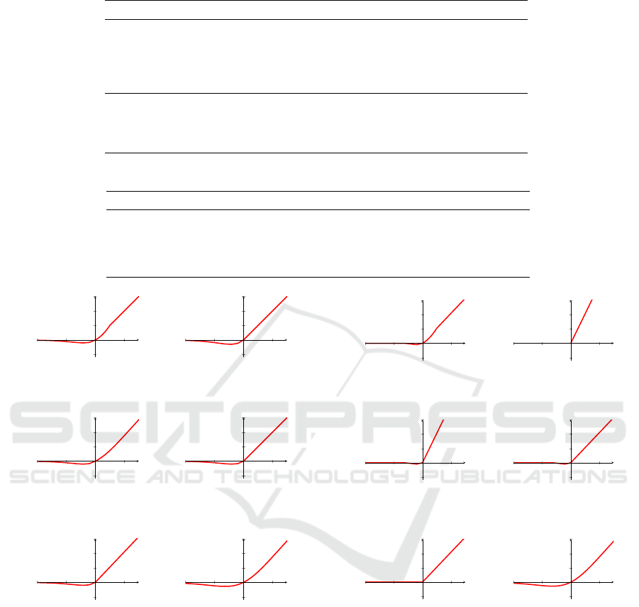
Table 2: Performance of top 5 evolved AFs for CIFAR-10 obtained using ResNet-20.

Accuracy Activation Function

1. 79.24% y(x < 0) = Softplus ×ELU and y(x ≥ 0) = ELU

2. 78.46% y(x < 0) = Softplus ×ELU and y(x ≥ 0) = max(ReLU, SeLU)

3. 78.39% y(x < 0) = Sigmoid ×SeLU and y(x ≥ 0) = min(Linear, ELU)

4. 77.72% y(x < 0) = Softplus ×ELU and y(x ≥ 0) = HardSigmoid ×Linear

5. 77.08% y(x < 0) = Softplus ×ELU and y(x ≥ 0) = Sigmoid ×ReLU

6. 78.51% y(x) = Swish

7. 73.00% y(x) = ELU

8. 71.98% y(x) = ReLU

9. 65.79% y(x) = SeLU

Table 3: Perfromance of top 5 AFs found by Random Search on CIFAR-10 obtained using ResNet-20.

Accuracy Activation Function

1. 76.03% y(x < 0) = SeLU × Sigmoid and y(x ≥ 0) = Sigmoid × Linear

2. 74.35% y(x < 0) = HardSigmoid and y(x ≥ 0) = HardSigmoid

3. 72.40% y(x < 0) = (ELU − HardSigmoid) and y(x ≥ 0) = (HardSigmoid − Linear)

4. 62.58% y(x < 0) = (Linear − ReLU) and y(x ≥ 0) = (Sigmoid − Sigmoid)

5. 51.65% y(x < 0) = HardSigmoid and y(x ≥ 0) = Sigmoid

−4 −2 2

−1

−4 −2 2

−1

y(x ≥ 0) = HardSigmoid × Linear

y(x < 0) = Softplus × ELU

y(x ≥ 0) = min(Linear,ELU)

y(x < 0) = Sigmoid × SeLU

−4 −2 2

−1

−4 −2 2

−1

y(x ≥ 0) = Sigmoid × ReLU

y(x < 0) = Softplus × ELU

y(x ≥ 0) = ELU

y(x < 0) = Softplus × ELU

−4 −2 2

−1

−4 −2 2

−1

y(x ≥ 0) = max(ReLU,SeLU)

y(x < 0) = Softplus × ELU

y(x) = Swish

Figure 7: Top 5 evolved AFs plus Swish for CIFAR-10.

Next, we run the same experiment using the VGG-

16 framework and show the results in Table 5. Even

though the AFs have not been trained for this archi-

tecture, we get competitive results. Similarly, we

get the best results again using the multiplication of

Softplus and ELU in negative part and HardSigmoid

and Linear in positive part (93.43%). These results

clearly show, that not only similar functions are evol-

ved, but that the results are competitive and outperfor-

ming the baseline in most cases.

Finally, we run experiments on CIFAR-100,

where the results for ResNet-56 and VGG-16 are

−4 −2 2

−1

−4 −2 2

−1

y(x ≥ 0) = HardSigmoid × SeLU

y(x < 0) = HardSigmoid × ELU

y(x ≥ 0) = (Linear + SeLU)

y(x < 0) = HardSigmoid × ReLU

−4 −2 2

−1

−4 −2 2

−1

y(x ≥ 0) = (Linear + SeLU)

y(x < 0) = Softplus × ELU

y(x ≥ 0) = SeLU

y(x < 0) = HardSigmoid × ELU

−4 −2 2

−1

−4 −2 2

−1

y(x ≥ 0) = SeLU

y(x < 0) = HardSigmoid × ReLU

y(x) = Swish

Figure 8: Top 5 evolded AFs plus Swish for CIFAR-100.

shown in Table 6 and Table 7, respectively. It can be

seen that the multiplication of ELU and HardSigmoid

in negative part and SeLU and HardSigmoid in po-

sitive part (73.84%) gives the best results for Res-

Net56. For VGG, the AF consisting of multiplication

of HardSigmoid and ReLU in the negative part and

SeLU in the positive part (71.36%) yields the best re-

sults. Again, the top 5 AFs compared to Swish are

illustrated in Figure 8. It can also be seen that com-

pared to CIFAR-10 the shapes of the evolved AFs are

different!

VISAPP 2019 - 14th International Conference on Computer Vision Theory and Applications

538

Table 4: Performance of top 5 evolved activation functions for CIFAR-10 based on ResNet-56.

Accuracy Activation Function

1. 93.00% y(x < 0) = Softplus ×ELU and y(x ≥ 0) = HardSigmoid ×Linear

2. 92.87% y(x < 0) = Sigmoid ×SeLU and y(x ≥ 0) = min(Linear, ELU)

3. 92.66% y(x < 0) = Softplus ×ELU and y(x ≥ 0) = Sigmoid ×ReLU

4. 92.38% y(x < 0) = Softplus ×ELU and y(x ≥ 0) = ELU

5. 92.27% y(x < 0) = Softplus ×ELU and y(x ≥ 0) = max(ReLU, SeLU)

6. 92.43% y(x) = ReLU

7. 91.45% y(x) = ELU

8. 91.43% y(x) = SeLU

6. 92.83% y(x) = Swish

Table 5: Performance of top 5 evolved AFs for Cifar10-VGG16.

Accuracy Activation Function

1. 93.43% y(x < 0) = Softplus × ELU and y(x ≥ 0) = HardSigmoid × Linear

2. 93.32% y(x < 0) = Softplus × ELU and y(x ≥ 0) = ELU

3. 93.18% y(x < 0) = Softplus × ELU and y(x ≥ 0) = max(ReLU,SeLU)

4. 93.14% y(x < 0) = Sigmoid × SeLU and y(x ≥ 0) = min(Linear,ELU)

5. 92.89% y(x < 0) = Softplus × ELU and y(x ≥ 0) = Sigmoid × ReLU

6. 93.00% y(x) = ReLU

7. 92.60% y(x) = ELU

8. 92.88% y(x) = SeLU

9. 93.00% y(x) = Swish

Table 6: Performance of top 5 evolved AFs for Cifar100-Resnet-56.

Accuracy Activation Function

1. 73.84% y(x < 0) = HardSigmoid × ELU and y(x ≥ 0) = HardSigmoid × SeLU

2. 73.81% y(x < 0) = HardSigmoid × ReLU and y(x ≥ 0) = SeLU + Linear

3. 73.77% y(x < 0) = Softplus × ELU and y(x ≥ 0) = SeLU + Linear

4. 73.52% y(x < 0) = HardSigmoid × ELU and y(x ≥ 0) = SeLU

5. 73.12% y(x < 0) = HardSigmoid × ReLU and y(x ≥ 0) = SeLU

5. 73.31% y(x) = ReLU

6. 72.58% y(x) = ELU

7. 71.57% y(x) = SeLU

8. 73.98% y(x) = Swish

Table 7: Performance of top 5 evolved AFs for Cifar100-VGG16.

Accuracy Activation Function

1. 71.36% y(x < 0) = HardSigmoid × ReLU and y(x ≥ 0) = SeLU

2. 71.28% y(x < 0) = Softplus × ELU and y(x ≥ 0) = SeLU + Linear

3. 70.95% y(x < 0) = HardSigmoid × ReLU and y(x ≥ 0) = SeLU + Linear

4. 70.22% y(x < 0) = HardSigmoid × ELU and y(x ≥ 0) = HardSigmoid × SeLU

5. 70.19% y(x < 0) = HardSigmoid × ELU and y(x ≥ 0) = SeLU

5. 70.74% y(x) = ReLU

6. 71.12% y(x) = ELU

7. 70.59% y(x) = SeLU

8. 71.23% y(x) = Swish

5 CONCLUSION

Even though deep learning approaches allow end-to-

end learning for a variety of applications, there are

still many parameters which need to be manually set.

An important parameter, which is often ignored, is the

choice of AFs. Thus, we tackled this problem and

studied the importance of AFs when learning DNNs

for classiﬁcation. In particular, we introduced a GP-

based evolving procedure to learn the best AF for a

given task. The presented results did not only show

competitive results but also that for different tasks dif-

ferent AFs are learned. In contrast to random sam-

pling, our approach guarantees that meaningful and

Learning Task-speciﬁc Activation Functions using Genetic Programming

539

competitive AFs are found. This is remarkable as

only very basic candidate solutions are provided (in

contrast to, e.g., Swish). Moreover, our approach is

adapting very well to different kinds of problems.

REFERENCES

Clevert, D., Unterthiner, T., and Hochreiter, S. (2016). Fast

and accurate deep network learning by exponential li-

near units (ELUs). In Proc. Int’l Conf. on Learning

Representations.

De Jong, K. A. (2006). Evolutionary Computation: A Uni-

ﬁed Approach. MIT press.

Elfwing, S., Uchibe, E., and Doya, K. (2018). Sigmoid-

weighted linear units for neural network function ap-

proximation in reinforcement learning. Neural Net-

works, 107:3–11.

Glorot, X., Bordes, A., and Bengio, Y. (2011). Deep sparse

rectiﬁer neural networks. In Pro. Int’l Conf. on Artiﬁ-

cial Intelligence and Statistics.

Goodfellow, I., Bengio, Y., and Courville, A. (2016). Deep

Learning. MIT Press.

Gulcehre, C., Moczulski, M., Denil, M., and Bengio, Y.

(2016). Noisy activation functions. In Proc. Int’l Conf.

on Machine Learning.

Hagg, A., Mensing, M., and Asteroth, A. (2017). Evolving

parsimonious networks by mixing activation functi-

ons. In Proc. Genetic and Evolutionary Computation

Conf.

Hancock, P. J. B. (1992). Pruning neural nets by genetic

algorithm. In Proc. Int’l Conf. on Artiﬁcial Neural

Networks.

Hayou, S., Doucet, A., and Rousseau, J. (2018). On the

selection of initialization and activation function for

deep neural networks. arXiv:1805.08266.

He, K., Zhang, X., Ren, S., and Sun, J. (2015). Delving deep

into rectiﬁers: Surpassing human-level performance

on imagenet classiﬁcation. In Proc. IEEE Int’l Conf.

on Computer Vision.

He, K., Zhang, X., Ren, S., and Sun, J. (2016). Identity

mappings in deep residual networks. In Proc. Euro-

pean Conf. on Computer Vision.

Hochreiter, S. (1998). The vanishing gradient problem du-

ring learning recurrent neural nets and problem so-

lutions. Int’l Journal of Uncertainty, Fuzziness and

Knowledge-Based System, 6(2):107–116.

Hornik, K. (1991). Approximation capabilities of mul-

tilayer feedforward networks. Neural Networks,

4(2):251–257.

Igel, C. (2003). Neuroevolution for reinforcement learning

using evolution strategies. In Proc. IEEE Congress on

Evolutionary Computation.

Klambauer, G., Unterthiner, T., Mayr, A., and Hochreiter,

S. (2017). Self-normalizing neural networks. In Ad-

vances on Neural Information Processing Systems.

Laurent, C., Pereyra, G., Brakel, P., Zhang, Y., and Ben-

gio, Y. (2016). Batch normalized recurrent neural net-

works. In Proc. IEEE Int’l Conf. on Acoustics, Speech

and Signal Processing.

LeCun, Y., Bengio, Y., and Hinton, G. (2015). Deep lear-

ning. Nature, 521:436–444.

Liu, H., Simonyan, K., Vinyals, O., Fernando, C., and Ka-

vukcuoglu, K. (2018). Hierarchical representations

for efﬁcient architecture search. In Proc. Int’l Conf.

on Learning Representations.

Loshchilov, I. and Hutter, F. (2016). CMA-ES for hyper-

parameter optimization of deep neural networks. In

Proc. Int’l Conf. on Learning Representations (Works-

hop track).

Maas, A. L., Hannun, A. Y., and Ng, A. Y. (2013). Rectiﬁer

nonlinearities improve neural network acoustic mo-

dels. In Proc. ICML Workshop on Deep Learning for

Audio, Speech and Language Processing.

Miikkulainen, R., Liang, J. Z., Meyerson, E., Rawal, A.,

Fink, D., Francon, O., Raju, B., Shahrzad, H., Navru-

zyan, A., Duffy, N., and Hodjat, B. (2017). Evolving

deep neural networks. CoRR, abs/1703.00548.

Mishkin, D. and Matas, J. (2017). All you need is a good

init. In Proc. Int’l Conf. on Learning Representations.

Mitchell, M. (1996). An Introduction to Genetic Algo-

rithms. MIT Press.

Montana, D. J. and Davis, L. (1989). Training feedforward

neural networks using genetic algorithms. In Proc.

Int’l Joint Conf. on Artiﬁcial Intelligence.

Nair, V. and Hinton, G. E. (2010). Rectiﬁed linear units

improve restricted boltzmann machines. In Proc. Int’l

Conf. on Machine Learning.

Pennington, J., Schoenholz, S. S., and Ganguli, S. (2018).

The emergence of spectral universality in deep net-

works. arXiv:1802.09979.

Qiang, X., Cheng, G., and Wang, Z. (2010). An overview of

some classical growing neural networks and new de-

velopments. In Proc. Int’l Conf. on Education Techno-

logy and Computer.

Ramachandran, P., Zoph, B., and V. Le, Q. (2018). Sear-

ching for activation functions. In Proc. Int’l Conf. on

Learning Representations (Workshop track).

Schaffer, J. D., Whitley, D., and Eshelman, L. J. (1992).

Combinations of genetic algorithms and neural net-

works: A survey of the state of the art. In Proc. Int’l

Workshop on Combinations of Genetic Algorithms

and Neural Networks.

Simonyan, K. and Zisserman, A. (2015). Very deep convo-

lutional networks for large-scale image recognition. In

Proc. Int’l Conf. on Learning Representations.

Stanley, K. O. and Miikkulainen, R. (2002). Evolving neu-

ral networks through augmenting topologies. Evoluti-

onary Computation, 10(2):99–127.

Suganuma, M., Shirakawa, S., and Nagao, T. (2017). A

genetic programming approach to designing convolu-

tional neural network architectures. In Proc. Genetic

and Evolutionary Computation Conference.

Sutskever, I., Martens, J., Dahl, G., and Hinton, G. (2013).

On the importance of initialization and momentum in

deep learning. In Proc. Int’l Conf. on Machine Lear-

ning.

Whitley, D. (2001). An overview of evolutionary algo-

rithms: Practical issues and common pitfalls. Infor-

mation and Software Technology, 43:817–831.

VISAPP 2019 - 14th International Conference on Computer Vision Theory and Applications

540