Comparison of Spatial Interpolation Methods based on Exposure
Assessments of Air Pollutants: A Case Study on Nuclear Substances
in Fukushima
Takahiro Otani
1
, Kunihiko Takahashi
1
, Ayano Takeuchi
2
and Mari Asami
3
1
Department of Biostatistics, Nagoya University Graduate School of Medicine, Showa-ku, Nagoya, Japan
2
School of Medicine, Keio University, Shinjuku-ku, Tokyo, Japan
3
Department of Environmental Health, National Institute of Public Health, Wako-shi, Saitama, Japan
Keywords: Spatial Interpolation, Exposure Assessment, Air Pollutants, Nuclear Substance.
Abstract: In response to accidents and disasters involving the proliferation of pollutants to the environment,
performing exposure assessments across a region of impact is important for evaluating health effects. Owing
to the typical unavailability of the spatially continuous data of pollutant concentrations immediately after
accidents, various spatial interpolation methods have been studied to assess exposures using limited
available data. In this study, we compared representative spatial interpolation methods based on the
estimation of the distributions of exposures through a case study of the Fukushima Daiichi nuclear disaster
initiated by the Great East Japan earthquake and subsequent tsunamis. The nearest neighbour method,
inverse distance weighted method, and ordinary kriging method were compared in the context of exposure
assessments. Even though estimated air dose rates were slightly different depending on the method used,
different interpolation methods produced significantly equivalent estimates of the distribution of cumulative
exposure over one year.
1 INTRODUCTION
Accidents and disasters involving the proliferation
of pollutants to the environment cause serious
problems for human health. As a response to
accidents, rapid and accurate exposure assessment is
required for evaluating health effects. For this
purpose, accurate spatially continuous data of
pollutant concentrations across a region of impact
are required. However, such data are typically not
available immediately following accidents. In such
cases, spatial interpolation is generally applied to
estimate values at unsampled points from limited
available data.
A motivating example is the proliferation of
radioactive pollutants due to the accident at the
Fukushima Daiichi Nuclear Power Plant (FDNPP)
initiated primarily by the tsunami following the
Tōhoku earthquake on 11 March, 2011. Extensive
survey meter measurements, airborne monitoring,
and vehicle-borne surveys have been conducted to
grasp the state of the spatial distribution of
pollutants (Fukushima Prefecture, 2011a; JAEA,
2013; MEXT, 2011a). In addition, exposure
assessments have been attempted for each residential
area based on these spatial data (Ishikawa, 2014;
Takahashi et al., 2014). On the other hand, the point
measurements of air dose rates were conducted
immediately after the accident across the region of
impact, and data were publicly reported (TEPCO,
2011; MEXT, 2011b; Fukushima Prefecture,
2011b). In a representative exposure assessment
conducted by National Institute of Radiological
Sciences (NIRS), the monitoring data scattered on
maps were converted to spatially continuous data
using the natural neighbour method (Akahane et al.,
2013). The estimation of the spatial distribution of
dose rate based on this data has been attempted
(Ishikawa et al., 2015). However, the problem with
this approach is that the estimate of the distribution
varies depending on the interpolation method used.
Various spatial interpolation methods have been
proposed to obtain spatially continuous data from
limited available information in an appropriate
manner (Lam, N. S. N. 1983; Li and Heap, 2008,
2014; Webster and Oliver, 2007). Additionally,
Otani, T., Takahashi, K., Takeuchi, A. and Asami, M.
Comparison of Spatial Interpolation Methods based on Exposure Assessments of Air Pollutants: A Case Study on Nuclear Substances in Fukushima.
DOI: 10.5220/0007523604150421
In Proceedings of the 12th International Joint Conference on Biomedical Engineering Systems and Technologies (BIOSTEC 2019), pages 415-421
ISBN: 978-989-758-353-7
Copyright
c
2019 by SCITEPRESS – Science and Technology Publications, Lda. All rights reserved
415

extensive comparative studies have been conducted
(Li and Heap, 2011). In the context of the evaluation
of human health, the effect of interpolation methods
on the accuracy of the estimation of exposures
should also be evaluated. Even though several
comparative studies exist (for example, Wong et al.,
2004), comparisons based on the influence of
interpolation methods on exposure assessment have
not been conducted in detail compared to the
evaluation of predicted concentration levels.
In this study, we examine how the estimation of
the distribution of exposure in a region changes
based on the method of spatial interpolation through
a case study of the accident at the FDNPP.
2 MATERIALS AND METHODS
In this study, we estimated the distributions of
cumulative exposure by
134
Cs and
137
Cs for each
municipality in Fukushima Prefecture for each age
category. Our procedure consisted of the following
two steps: convert monitoring data to spatially
continuous data using interpolation methods and
estimate the distribution of exposure using the
continuous data based on an external exposure
model.
2.1 Monitoring Data
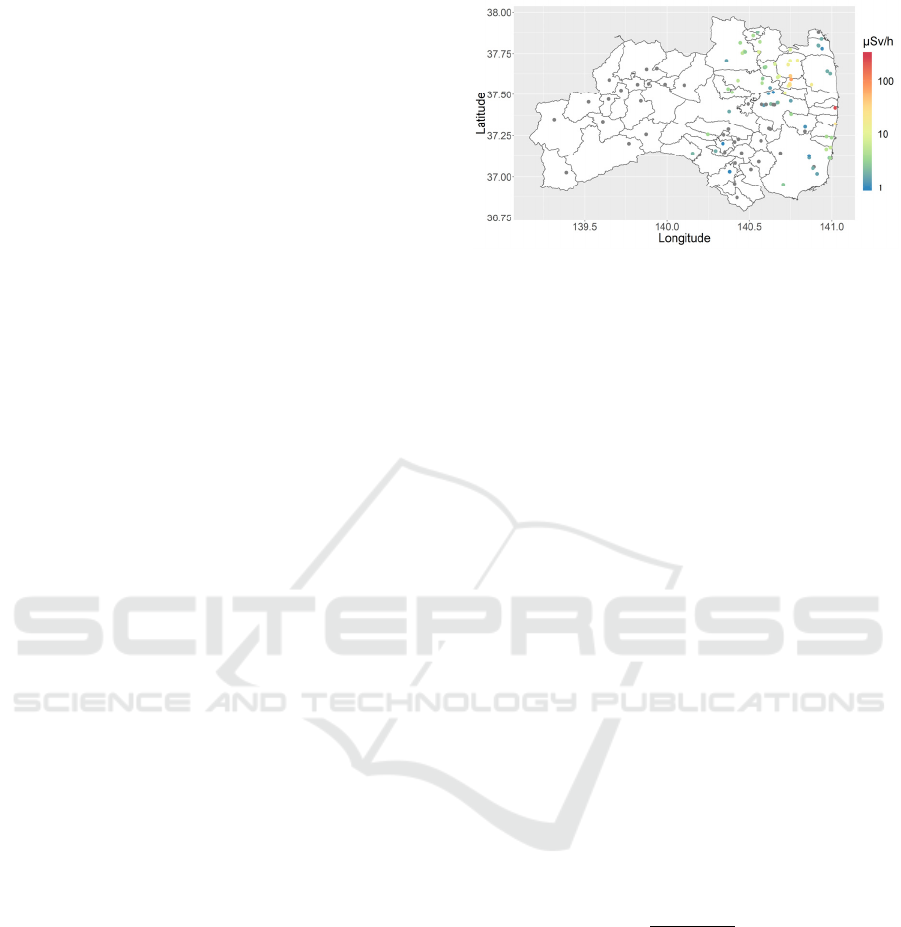
Figure 1 shows a map of Fukushima Prefecture with
monitoring data. The data consist of 113 air dose
rates measured on 22 March, 2011 and published
online (TEPCO, 2011; MEXT, 2011b; Fukushima
Prefecture, 2011b).
2.2 Interpolation Methods
The following three representative interpolation
methods were compared in this study: the (i) nearest
neighbour (NN) method, (ii) inverse distance
weighted (IDW) method, and (iii) ordinary kriging
(OK) method (Lam, N. S. N. 1983; Li and Heap,
2008, 2014, Webster and Oliver, 2007). Note that
we applied logarithm transformation to the
monitoring data before interpolation because the
distribution of dose rates was skewed.
2.2.1 Nearest Neighbour Method
The NN method predicts the dose rate at an
unsampled point based on the value of the nearest
sample by drawing perpendicular bisectors between
sampled points, forming Voronoi polygons (Li and
Figure 1: Air dose rates measured on March 22, 2011.
Note that points with rates of <1 μSv/h are coloured in
grey.
Heap, 2008; Webster and Oliver, 2007). Let ̂
be
the estimated air dose rate at unsampled points .
The estimates by the NN method are the values at
the nearest single sampled data points,
, that is,
̂
=
.
(1)
2.2.2 Inverse Distance Weighted Method
The IDW method estimates the values at unsampled
points using a linear combination of the values at
sampled points weighted by an inverse function of
the distance from the point of interest to the sampled
points. The estimated value is
̂
=
.
(2)
Here, the weight,
, is determined assuming that the
sampled points closer to an unsampled point in
terms of their values are more similar to it compared
to those further away. The weights can be expressed
as
=
1
⁄
∑
1
⁄
(3)
where
is the distance between
and
, is a
power parameter, and represents the number of
sampled points used for estimation. In this study, we
set =2 and =5.
2.2.3 Ordinary Kriging Method
Similar to the IDW method, the OK method
estimates the dose rates at unsampled points by a
weighted averaging of neighbouring samples. The
correlations among neighbouring values are
modelled as a function of the distance between the
HEALTHINF 2019 - 12th International Conference on Health Informatics
416

points, which is described by a variogram (Webster
and Oliver, 2007).
An empirical variogram can be computed from
sampled data using the following expression:
=
1
2
(4)
where
is the estimated semivariogram at
separation distance , of which there are
pairs.
The weight,
, is determined such that the variance
of estimated values is minimised. The method
consists of the following two steps: fitting a function
to the empirical variogram such that semivariograms
can be computed at all separation distances and
computing
such that estimation variance is
minimised. In this study, we used the spherical
specification as the fitting function.
2.3 Estimation of Cumulative Exposure
We estimated the distribution of cumulative
exposure one year after the accident for each
municipality in Fukushima Prefecture based on the
Monte Carlo sampling method by referring to
existing studies (Takahashi et al., 2014).
2.3.1 External Exposure Model
In this model, cumulative exposure is estimated
considering only the attenuation due to the physical
half-life of radioactive caesium to be variable with
time. Let be the municipality of interest and be
the point in at which the predicted air dose rate,
̂
, at time is available. The cumulative
exposure one year after the accident is estimated by
summing the cumulative exposure due to
radionuclide as
E
,
=
⋅Φ
⋅
⋅Φ
⋅1
⋅
(5)
where Φ
is the dose-rate conversion factor of
radionuclide , is the outdoor staying time ratio for
age category ,
is the proportion of building type
in Fukushima Prefecture, and
is the shielding
factor for each type of building. In addition,
is
the cumulative exposure due to radionuclide , and it
is expressed as
=
⋅
.
(6)
As the purpose of this study is to estimate the
cumulative exposure one year after the accident, the
integration interval is from 0 to 1.
Here, we assumed that
can be determined
only by the deposition amounts of
134
Cs and
137
Cs at
time . The initial deposition amount for each
radionuclide can be obtained as
=
̂
Φ
Φ
(7)
=
̂
Φ
Φ
(8)
where Φ
and Φ
are the dose-rate conversion
factors of
134
Cs and
137
Cs, respectively, and is the
activity ratio of
134
Cs/
137
Cs at =0.
In this model, the outdoor staying time ratio, ,
is derived from a log-normal distribution so that the
5
th
percentile and the 50
th
percentile of outdoor
staying time for each age category are matched with
those of USEPA (2011). Random numbers were
generated corresponding to each point in and
multiplied by the cumulative exposure at each point.
2.3.2 Parameters of the Model
We determined the parameters of the model by
referring to existing studies and technical documents
(IAEA, 2000; Merz, 2013; Statistics Bureau 2008;
USEPA, 2011). The parameters are shown in Tables
1 and 2. The dose-rate conversion factors and decay
constants of
134
Cs and
137
Cs and shielding factors
were based on a technical document (IAEA, 2000).
Table 1: Parameters used in this study.
Description Value
Activity ratio of
134
Cs/
137
Cs at t = 0 1
Dose-rate conversion factor of
134
Cs
[(mSv/h)/(kBq/m
2
)]
5.4E-06
Dose-rate conversion factor of
137
Cs
[(mSv/h)/(kBq/m
2
)]
2.1E-06
Decay constant of
134
Cs 0.346
Decay constant of
137
Cs 0.0231
Proportion of wooden building 0.37
Proportion of non-wooden building 0.63
Shielding factor of wooden building 0.4
Shielding factor of non-wooden building 0.2
Comparison of Spatial Interpolation Methods based on Exposure Assessments of Air Pollutants: A Case Study on Nuclear Substances in
Fukushima
417

Table 2: Distribution of outdoor staying time (hours/day)
for each age category (USEPA, 2011).
Age category 5
th
percentile 50
th
percentile
0–1 0.05 0.70
1–6 0.08 2.10
7–15 0.01 3.00
16– 0.02 4.30
In addition, the activity ratio at =0 was based on
an existing study (Merz, 2013). As the proportions
of wooden and non-wooden buildings are different
depending on the region in Japan, we used the
published ratios of Fukushima Prefecture (Statistics
Bureau 2008).
In addition, points were selected from a basic
square grid with a size of approximately 1 km
2
(Statistics Bureau 2018). was 0.027, which
corresponds to the date of monitoring, i.e. March 22,
2011.
2.4 Comparison with Airborne Survey
We compared the estimated cumulative exposure
with the estimates obtained from the results of the
fourth airborne monitoring survey conducted from
22 October, 2011 to 5 November, 2011 (MEXT,
2011c) to assess the validity of our method. The
survey data consisted of radioactive caesium
deposition densities at the median points of quarter
grid squares with a size of approximately 250 m
2
(Statistics Bureau 2018). Cumulative exposure was
estimated based on the model described in
Takahashi et al., 2014.
3 RESULTS
First, we obtained the spatially continuous data of air
dose rates from the monitoring data shown in Figure
1 using the three interpolation methods. Figure 2
shows the spatial distributions of air dose rates in
Fukushima Prefecture estimated by each method.
Different estimations were produced depending on
the method used, particularly in areas close to the
FDNPP. Among these, the estimates by the NN
method were higher than those by the other methods
because only monitoring data with significant air
dose rates obtained at the FDNPP (TEPCO, 2011)
were available in this area and the NN directly used
these data as predicted values.
Based on these results, we estimated the
distributions of cumulative exposure for each
municipality in Fukushima Prefecture using the
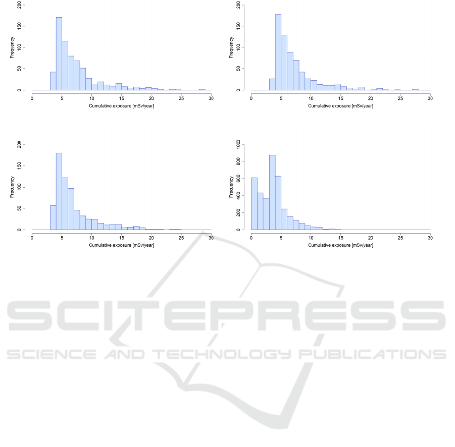
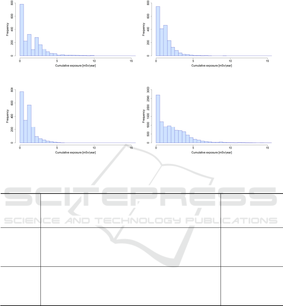
model described in section 2.3. Figures 3 and 4 show
the histograms of the estimated cumulative exposure
in municipalities with comparatively high doses (A)
and low doses (B) for ages 1–6. Here, we also
describe the estimates based on the data from the
airborne monitoring survey (MEXT, 2011c;
Takahashi et al., 2014). In contrast to the estimates
of air dose rate (Figure 2), different interpolation
methods did not produce significantly different
estimations in most parts of Fukushima Prefecture.
(a) Nearest neighbour method
(b) Inverse distance weighted method
(c) Ordinary kriging method
Figure 2: Estimated distributions of air dose rates in
Fukushima Prefecture on 22 March, 2011. Note that areas
with dose rates of <1 μSv/h are coloured in grey. A and B
are municipalities with comparatively high doses and low
doses, respectively.
B
A
A
B
B
A
HEALTHINF 2019 - 12th International Conference on Health Informatics
418

(a) Nearest neighbour method (b) Inverse distance weighted method
(c) Ordinary kriging method (d) Airborne monitoring
Figure 3: Histograms of the estimated grid-wise cumulative exposure in municipality A for ages 1–6.
In contrast, our estimates were slightly different
from the results of the airborne monitoring survey.
For municipality A, even though the estimate from
the survey suggested the existence of a low exposure
of <3 mSv/year, our estimates could not express
such a low exposure. For municipality B, our
estimates suggested that almost all regions had low
exposure while the distribution of airborne
monitoring result indicated high exposure. However,
the estimates of the mode were comparable in both
municipalities. These results imply that the estimates
of cumulative exposure for most regions in each
municipality are almost the same regardless of the
method used. Of the three interpolation methods, the
mode of the OK method was the most similar to the
airborne monitoring.
Owing to these results, the percentiles of our
estimates were different from the results of the
airborne monitoring survey. Table 3 shows 50
th
and
90
th
percentiles of the estimated cumulative
exposure in municipalities A and B for each age
category. There was an approximately twofold
difference between these estimates and the results of
this survey. The differences varied depending on the
municipality, e.g. our estimates were higher than the
existing estimates in municipality A and lower in
municipality B.
4 CONCLUSIONS
In this study, we compared three representative
spatial interpolation methods in the context of the
exposure assessments of air pollutants through a
case study of the Fukushima Daiichi nuclear
disaster. Even though estimated air dose rates were
slightly different depending on the method used,
different interpolation methods did not produce
significantly different estimates of the distribution of
cumulative exposure over one year. On the contrary,
the estimates of exposure were different from the
results of the airborne monitoring survey, even
though they were of the same order of magnitude.
As the method based on spatial interpolation
estimates the air dose rate using only acquired data,
such bias might be strong when measurement points
are not dense. It is crucial to perform measurement
densely, particularly in areas where the dose rate
difference is large depending on location.
Even though we only considered estimating the
grid-wise cumulative exposure for each municipality
in this study, the estimated distribution can also be
used to estimate the exposure population. More
appropriate exposure assessment might be conducted
using demographics.
Comparison of Spatial Interpolation Methods based on Exposure Assessments of Air Pollutants: A Case Study on Nuclear Substances in
Fukushima
419

(a) Nearest neighbour method (b) Inverse distance weighted method
(c) Ordinary kriging method (d) Airborne monitoring
Figure 4: Histograms of the estimated grid-wise cumulative exposure in municipality B for ages 1–6.
Table 3: Estimated grid-wise cumulative exposure [mSv/year] in municipalities A and B.
Area Age Nearest Neighbour
Inverse Distance
Weighted
Ordinary Kriging
Airborne Monitoring
(Takahashi et al. 2014)
50
th
percentile
95
th
percentile
50
th
percentile
95
th
percentile
50
th
percentile
95
th
percentile
50
th
percentile
95
th
percentile
A 0–1 5.2 12.7 5.3 10.7 5.1 9.8 3.2 5.7
1–6 6.2 15.6 6.1 15.5 5.7 14.6 3.4 8.0
7–15 6.0 16.8 5.6 16.5 5.3 15.2 3.3 8.4
16– 6.4 17.6 5.9 15.9 5.5 13.0 3.4 8.6
B 0–1 1.0 3.3 0.9 2.2 0.8 1.9 1.5 4.5
1–6 1.1 4.5 0.9 3.1 0.9 2.8 1.7 5.9
7–15 1.0 4.8 0.9 3.2 0.9 2.8 1.6 6.0
16– 1.0 4.9 0.9 3.3 0.9 3.3 1.7 6.2
As demonstrated in this study, when spatial
interpolation is performed from the measured data of
pollutant concentration levels, the estimation result
varies depending on the method used. While the
evaluation of predicted concentration levels is
naturally crucial, it is also necessary to consider the
magnitude of change in exposure evaluation for
selecting an interpolation method and interpreting
results.
ACKNOWLEDGEMENTS
This work was supported by the Environment
Research and Technology Development Fund (S-17)
of the Ministry of the Environment, Japan.
HEALTHINF 2019 - 12th International Conference on Health Informatics
420

REFERENCES
Akahane, K., Yonai, S., Fukuda, S., et al. 2013. NIRS
external dose estimation system for Fukushima
residents after the Fukushima Dai-ichi NPP accident.
Scientific Reports. 3, pp. 1–6.
Fukushima Prefecture 2011a. Environmental Radiation
Monitoring in Mesh Survey, http://www.pref.
fukushima.lg.jp/sec/16025d/mesh-1.html (in Japanese:
Accessed on 4 November 2018).
Fukushima Prefecture 2011b. Past radiation monitoring
results, http://www.pref.fukushima.lg.jp/sec/16025d/
kako-monitoring.html (in Japanese: Accessed on 4
November 2018).
International Atomic Energy Agency (IAEA) 2000.
Generic procedures for assessment and response
during a radiological emergency (IAEA-TECDOC-
1162), IAEA. Vienna, Austria.
Ishikawa, T. 2014. A brief review of dose estimation
studies conducted after the Fukushima Daiichi Nuclear
Power Plant accident. Radiation Emergency Medicine.
3, pp. 21–27.
Ishikawa, T., Yasumura, S., Ozasa, K., et al. 2015. The
Fukushima Health Management Survey: Estimation of
external doses to residents in Fukushima Prefecture.
Scientific Reports. 5, pp. 1–11.
Japan Atomic Energy Agency (JAEA) 2013. The Second
Survey on the Distribution Condition of Radioactive
Substances by MEXT due to the Accident at TEPCO’s
Fukushima Dai-ichi NPP, Report on the Preparation
of Distribution Maps of Radiation Doses, etc. (Part 1).
JAEA, Ibaraki, Japan (in Japanese).
Lam, N. S. N. 1983. Spatial interpolation methods: A
review. Cartography and Geographic Information
Science. 10(2), pp. 129–150.
Li, J., Heap, A. D. 2008. A review of spatial interpolation
methods for environmental scientists. Geoscience
Australia, Record 2008/23.
Li, J., Heap, A. D. 2011. A review of comparative studies
of spatial interpolation methods in environmental
sciences: Performance and impact factors. Ecological
Informatics, 6(3-4), pp. 228–241.
Li, J., Heap, A. D. 2014. Spatial interpolation methods
applied in the environmental sciences: A review.
Environmental Modelling and Software. 53, pp. 173–
189.
Merz, S., Steinhauser, G., Hamada, N. 2013.
Anthropogenic radionuclides in Japanese food:
Environmental and legal implications. Environmental
Science and Technology. 47(3), pp. 1248–1256.
Ministry of Education, Culture, Sports, Science and
Technology (MEXT) 2011a. Results of Airborne
Monitoring by the MEXT and the U.S. Department of
Energy, MEXT. Tokyo, Japan.
Ministry of Education, Culture, Sports, Science and
Technology (MEXT) 2011b. Readings at reading post
out of 20 km zone of TEPCO Fukushima Dai-ichi
NPP, http://radioactivity.nsr.go.jp/ja/contents/3000/
2924/24/1303995_2310.pdf (in Japanese: Accessed on
4 November 2018).
Ministry of Education, Culture, Sports, Science and
Technology (MEXT) 2011c. Results of the Fourth
Airborne Monitoring Survey by MEXT, MEXT. Tokyo,
Japan.
Statistics Bureau 2008. 2008 Housing and Land Survey,
Statistics Bureau. Tokyo, Japan.
Statistics Bureau 2018. Ministry of Internal Affairs and
Communications website – Grid Square Statistics,
http://www.stat.go.jp/english/data/mesh/index.html
(Accessed on 4 November 2018).
Takahashi, K., Izumi, S., Takeuchi, A. 2014.
Epidemiologic studies with location information and
their statistical methods. Proceedings of the Institute
of Statistical Mathematics. 62(1), pp. 3–24 (in
Japanese).
Tokyo Electric Power Company (TEPCO) 2011.
Fukushima Daiichi information – Observation data,
https://www7.tepco.co.jp/responsibility/decommission
ing/1f_newsroom/data/index-e.html (Accessed on 4
November 2018).
United States Environmental Protection Agency (USEPA)
2011. Exposure Factors Handbook 2011 Edition,
USEPA. Washington, D.C.
Webster, R., Oliver, M. A. 2007. Geostatistics for
Environmental Scientists. John Wiley & Sons, Ltd.
Chichester, UK.
Wong, D. W., Yuan, L., Perlin, S. A. 2004. Comparison of
spatial interpolation methods for the estimation of air
quality data. Journal of Exposure Analysis and
Environmental Epidemiology. 14(5), pp. 404–415.
Comparison of Spatial Interpolation Methods based on Exposure Assessments of Air Pollutants: A Case Study on Nuclear Substances in
Fukushima
421
