
A Multi-objective Approach to the Optimization of Home Care Visits
Scheduling
Filipe Alves
1,2
, Lino Costa
3
, Ana Maria A. C. Rocha
3
, Ana I. Pereira
1,2
and Paulo Leit
˜
ao
1
1
Research Centre in Digitalization and Intelligent Robotics (CeDRI), Instituto Polit
´
ecnico de Braganc¸a, Braganc¸a, Portugal
2
Algoritmi R&D Centre, University of Minho, Braga, Portugal
3
Department of Production and Systems, Algoritmi R&D Centre, University of Minho, Braga, Portugal
Keywords:
Home Health Care, Multi-objective, Scheduling, Optimization.
Abstract:
Due to the increasing of life expectancy in the developed countries, the demand for home health care services is
growing dramatically. Usually, home services are planned manually and lead to various optimization problems
in their activities. In this sense, health units are confronted with appropriate scheduling which may contain
multiple, often conflicting, objectives such as minimizing the costs related to the traveling distance while
minimizing the traveling time. In order to analyze and discuss different trade-offs between these objectives, it
is proposed a multi-objective approach to home health care scheduling in which the problem is solved using
the Tchebycheff method and a Genetic algorithm. Different alternative solutions are presented to the decision
maker that taking into account his/her preferences chooses the appropriate solution. A problem with real data
from a home health care service is solved. The results highlight the importance of a multi-objective approach
to optimize and support decision making in home health care services. Moreover, this approach provides
efficient and good solutions in a reasonable time.
1 INTRODUCTION
Over the last decade, the increased life expectancy
resulted in increased demand for Home Health Care
(HHC) (Fikar and Hirsch, 2017). In this sense, the
number of people who needs home care services
are consequently growing worldwide (Nickel et al.,
2012). Therefore, health units that provide home care
services need to optimize their activities in order to
meet the constantly increasing demand for home care
services (Koeleman et al., 2012). This is usually due
to the manual planning of home care visits, making
it a time and effort consuming task that often leads
to inefficient solutions. Thus, the operation manage-
ment within the HHC turns to be very hard because
of the high number and diversity of human and mate-
rial resources that participate in the process of home
care and the criteria to be optimized (Benzarti et al.,
2013). Regarding the literature in this field, there
are some issues relevant to the home care visits sche-
dule. Some authors present an overview of works re-
lated to HHC (Benzarti et al., 2010). The work of
Yalc¸ındag et al. (2011) besides presenting the par-
ticular scheduling of visits also lists the well-known
routing problems in HHC. The problems that address
static multi-vehicle routing and assignment are a very
well-known and researched topic in Operations Re-
search (Baker and Ayechew, 2003; Toth and Vigo,
2014). In the context of HHC, these problems consist
in scheduling vehicles with nurses to patients (Bred-
str
¨
om and R
¨
onnqvist, 2008), in order to determine the
best order and time that visits should be performed. In
this subject, some works propose an approach to find
the best schedule, minimizing the costs (Nguyen and
Montemanni, 2013). On the other hand, some prob-
lems were modeled to be solved by the “branch and
price” algorithm (Rasmussen et al., 2012). Recently,
Alves et al. (2018) proposed an approach using the ge-
netic algorithm to solve the scheduling of home visits
as a single objective optimization problem. The work
of Allaoua et al. (2013) also presents the home care
scheduling problem as a single objective by minimi-
zing the travel cost or the travel time.
In this context, it is important to mention that
new research in HHC is being targeted with multi-
objective optimization approaches (Ombuki et al.,
2006; Pasia et al., 2007). For example, Braekers et al.
(2016) presents an approach that analyzes the trade-
off between costs and client inconvenience, using a
meta-heuristic algorithm based on multi-directional
Alves, F., Costa, L., Rocha, A., Pereira, A. and Leitão, P.
A Multi-objective Approach to the Optimization of Home Care Visits Scheduling.
DOI: 10.5220/0007565704350442
In Proceedings of the 8th International Conference on Operations Research and Enterprise Systems (ICORES 2019), pages 435-442
ISBN: 978-989-758-352-0
Copyright
c
2019 by SCITEPRESS – Science and Technology Publications, Lda. All rights reserved
435

local search. Thus, multi-objective solution proce-
dures derive a set of Pareto optimal solutions that are
not yet common in HHC scheduling (Braekers et al.,
2016; Gayraud et al., 2013).
In this work, the home health care scheduling
problem is formulated as a multi-objective problem
and an instance with real data is solved. Conflicting
objectives, such as costs, distances or unexpected and
inconvenient events are important to be considered.
The developed approach and model try to handle the
objectives of home care services and the patient’s ob-
jectives. To achieve this goal, additional costs related
to the travelling time and the travelling distance as
well as the waiting time are minimized. The obtained
solutions assist the decision making process in terms
of these objectives. As a result of using the Tcheby-
cheff method and a Genetic algorithm, multiple alter-
natives are presented to decision makers that can in-
spect benefits and trade-offs to derive daily schedules
based on individual or mutual preferences.
The paper is organized as follows. In Section 2,
the assumptions and the mathematical formulation of
the problem are presented. The multi-objective op-
timization approach is described in Section 3. Sec-
tion 4 presents the results for a case study based on
real data. In this section, the results are also analyzed
and discussed. Finally, some conclusions and future
work are drawn in Section 5.
2 PROBLEM DEFINITION
The problem arises when it is necessary to overcome
the difficulties that HHC services entail, such as the
vehicles delay that consequently cause bad schedules
with no viable replacement options and consequently
increase the expenses of Health Unit.
However, it is important to define the general char-
acteristics of the problem, such as the number and
characterization of health professionals, the number
of vehicles available, the number of patients and treat-
ments they need, locations that can be traveled and
their distances. This information and data allow to
create a mathematical formulation of the problem, as
an attempt to reduce the time spent on visits and con-
sequently the reduction of costs.
2.1 Assumptions
The vehicle scheduling carries out home care visits
in order to perform the necessary treatments for pa-
tients belonging to a Health Unit. This problem was
modeled, considering the number of vehicles involved
in the teams and the patients who request this type
of health care. Thus, considering a Health Unit in
Braganc¸a, with a domiciliary team that provides home
care to patients that require different types of treat-
ments, all the entities involved in the problem were
identified.
Consider the following information:
• the trips duration and distances between the dif-
ferent locations;
• the time of travel, in the same location, to visit
different patients;
• the distance, in the same location, to visit different
patients;
• the list and duration of treatments are known for
each patient (defined and provided by the Health
Unit);
• the number of patients who need health care, and
who are assigned to days of home visits, are
known in advance;
• the number of vehicles available;
• all visits begin and end at the Health Unit.
The mathematical formulation considers the fol-
lowing sets:
• P is the set of np ∈ N patients that receive home
care visits, P = {p
1
, . . . , p
np
};
• V is the set of nv ∈ N vehicles that perform home
care visits, V = {v
1
, . . . , v
nv
};
• L is the set of nl ∈ N locations for home care vis-
its, L = {l
1
, . . . , l
nl
};
• T is the set of nt ∈ N treatments required by pa-
tients, T = {t
1
, . . . ,t
nt
};
• R
i
, where i ∈ {1, . . . , nt}, is the set of nr
i
∈ N pa-
tients that receive the treatment i, R
i
⊂ P;
• Q
i
, where i ∈ {1, . . . , nl}, is the set of nl
i
∈ N pa-
tients that reside in location i, Q
i
⊂ P.
The parameters of the model are:
• D
nl×nl
is the matrix of distances between the nl
locations (the diagonal indicate the distance re-
quired to visit different patients in the same lo-
cation);
• H
nl×nl
is the matrix of time required to travel bet-
ween the nl locations (the diagonal indicate the
time required to visit different patients in the same
location);
• O
nt×1
is the vector of times required to apply each
of the nt treatments to patients.
Taking into account the information regarding
these sets and parameters, a vehicle scheduling op-
timization problem can be formulated to reduce the
time spent on visits and the costs.
ICORES 2019 - 8th International Conference on Operations Research and Enterprise Systems
436

2.2 Mathematical Formulation
The goal is to find the vehicle scheduling solution that
minimizes, simultaneously, the time spent on visits
and costs. A solution for this problem can be ex-
pressed by the vector x of dimension n = 2 × np with
the following structure:
x = (y, z) = (y
1
, ..., y
np
, z
1
, ..., z
np
)
where the patient y
i
∈ P will be visited by the vehi-
cle z
i
∈ V , for i = 1, . . . , np. In this vector, y
i
6= y
j
for
∀i 6= j with i = 1, . . . , np, j = 1, . . . , np. Therefore, for
a given x it is possible to define the vehicles schedu-
ling taking into account the order of the components
of x. For instance, consider a scheduling problem
with np = 5 patients to be visited by nv = 3 vehicles.
for P = {p
1
, p
2
, p
3
, p
4
, p
5
} and V = {v
1
, v
2
, v
3
}, the
vector x = (4, 3, 1, 2, 5, 2, 3, 2, 1, 1) means that patients
p
4
, p
3
, p
1
, p
2
and p
5
will be visited by vehicles v
2
,
v
3
, v
2
, v
1
and v
1
, respectively. Thus, vehicle v
1
will
visit patients p
2
and p
5
; vehicle v
2
will visit patients
p
4
and p
1
; and vehicle v
3
will visit patient p
3
. For
a vehicle schedule x, the functions t
l
(x) and d
l
(x),
for l = 1, .., nv, give the total time and total distance
required to perform all visits of the vehicle l, respec-
tively. The two objective functions are defined as
f
1
(x) = max
l=1,...,nv
t
l
(x) (1)
f
2
(x) = max
l=1,...,nv
d
l
(x) (2)
which represent, respectively, the maximum time and
maximum distance spent by all the vehicles to carry
out all the visits. Then, the optimization problem can
be defined as:
min
x∈Ω
f
1
(x), f
2
(x)
(3)
where x ∈ Ω is the decision variable space and Ω =
{(y, z) : y ∈ P
np
, z ∈ V
np
and y
i
6= y
j
for all i 6= j} is
the feasible set.
3 MULTI-OBJECTIVE
APPROACH
The vehicle scheduling problem formulated previ-
ously is a multi-objective problem, since the objec-
tives conflict each other. The goal is to find the set
of feasible trade-off solutions x that simultaneously
minimize f
1
(x) and f
2
(x) in order to facilitate the de-
cision maker select the solution according to his/her
preferences.
3.1 Multi-objective Optimization
When several conflicting objectives are optimized at
the same time, the search space becomes partially
ordered. In such scenario, solutions are compared
on the basis of the Pareto dominance. Without loss
of generality, consider a multi-objective optimization
problem where m objectives are to be minimized, for
two solutions a and b from the feasible set Ω, a so-
lution a is said to dominate a solution b (denoted by
a ≺ b) if:
∀i ∈ {1, . . . , m} : f
i
(a) ≤ f
i
(b)∧
∃ j ∈ {1, . . . , m} : f
j
(a) < f
j
(b).
(4)
Since solutions are compared against different ob-
jectives, there is no longer a single optimal solution
but a set of optimal solutions, generally known as
the Pareto optimal set. This set contains equally im-
portant solutions representing different trade-offs be-
tween the given objectives and can be defined as:
P S = {x ∈ Ω |@y ∈ Ω : y ≺ x}. (5)
The images of the solutions of the Pareto optimal
set define a Pareto front in the objective space. This
Pareto front allow to identify the trade-offs between
solutions and therefore facilitate the decision making.
3.2 Tchebycheff Scalarization Method
Approximating the Pareto optimal set is the main
goal of a multi-objective optimization algorithm. The
scalarization methods can be used to obtain an ap-
proximation to the Pareto-optimal set (Miettinen,
2012) such as:
• the weighted sum method, where the weighted
linear combination of the objectives is minimized;
• the ε-constraint method, in which one of the ob-
jectives is minimized and the others are included
as constraints;
• the minimization of a weighted distance to a
reference point, e.g., the weighted Tchebycheff
method.
When using these scalarization methods, the
multi-objective problem is transformed into a sin-
gle objective optimization problem that have to be
solved using single objective optimization algorithms.
There must be some care in choosing the scalariza-
tion method since the weighted sum method does not
allow to achieve solutions belonging to non-convex
regions of the Pareto front. On the other hand, in
the ε-constraint method is difficult to properly fix
the limits of the constrained objectives. Since the
vehicle scheduling problem is a non-continuous and
A Multi-objective Approach to the Optimization of Home Care Visits Scheduling
437

non-convex problem, then the weighted Tchebycheff
method was adopted to solve this problem. The main
goal is to approximate the optimal Pareto solutions
that represent different trade-offs between the objec-
tives. In the weighted Tchebycheff method the L
∞
norm (i.e., minimization of the maximum difference)
is used. This distance is computed to a reference point
(or aspiration levels). The weighting coefficients al-
low to obtain different trade-offs and lead with differ-
ent scaling factors of each objective. In this method,
the scalarized function is a weighted function based
on the Tchebycheff metric, to the reference point. The
weighted problem of Tchebycheff is given as follows
(Miettinen, 2012):
minmax[w
i
| f
i
(x) − z
?
i
|] (6)
where w
i
are the weighting coefficients for objective
i, z
?
i
are the components of a reference point. An ap-
proximation to the ideal vector can be used as refer-
ence point z
?
= (z
?
1
, . . . , z
?
m
) = (min f
1
, . . . , min f
m
).
This approach can be implemented as an a pri-
ori technique in which the reference point and the
weights are defined by the decision maker before the
search. There are some drawbacks in this approach
namely, the difficulty to define properly weights and
aspiration levels that reflect the decision maker pre-
ferences. Other perspective is to implement an a pos-
teriori technique in which the decision making pro-
cess takes place after the search. In this case, the re-
ference point is defined as the ideal solution and the
weights are uniformly varied. In this manner, after the
search, a set of Pareto optimal solutions is presented
as alternatives and the decision maker can identify the
compromises and choose according to his/her prefer-
ences. Thus, due to its ability to solve this kind of
problems, a Genetic algorithm was assumed.
3.3 Genetic Algorithm
A Genetic algorithm (GA) (Holland, 1992) is used
to solve each single objective optimization problem
that results of the weighted Tchebycheff method.
GA is inspired by the natural biological evolution,
uses a population of individuals and new individu-
als are generated by applying the genetic operators of
crossover and mutation.
Genetic algorithm are particularly well suited to
solve vehicle scheduling problem that is non-convex
with discrete decision variable and couple with the
combinatorial nature of the search space. The fle-
xibility of representation of the solutions and genetic
operators allow to handle hard constraints.
The GA used in this work is summarized in Al-
gorithm 1. Initially, a population of N
pop
individuals
is randomly generated. Each individual in the popu-
lation is a vector of decision variables x. Afterwards,
each generation, crossover and mutation operators are
applied to generate new solutions. These genetic op-
erators were designed in order to guarantee that new
solutions are feasible.
The best individuals in the population have a high
probability of being selected to generate new ones by
crossover and mutation. Therefore, the good features
of the individuals tend to be inherited by the offspring.
In this manner, population converges towards better
solutions (Ghaheri et al., 2015). The iterative proce-
dure terminates after a maximum number of iterations
(NI) or a maximum number of function evaluations
(NFE).
Algorithm 1: Genetic Algorithm.
1: P
0
= initialization: randomly generate a population of N
pop
individuals.
2: Set iteration counter k = 0.
3: while stopping criterion is not met do
4: P
0
= crossover(P
k
): apply crossover procedure to individuals in
population P
k
.
5: P
00
= mutation(P
k
): apply mutation procedure to individuals in pop-
ulation P
k
.
6: P
k+1
= selection(P
k
∪ P
0
∪ P
00
): select the N
pop
best individuals of
P
k
∪ P
0
∪ P
00
.
7: Set k = k + 1.
8: end while
3.4 Multi-objective Optimization
Framework
Figure 1 describes and illustrates the entire frame-
work of this multi-objective approach.
Genetic
Algorithm
Metric
Tchebychev
Multi-objective
Problem
Objective 1
(Time)
Objective 2
(Distance)
[ w, ref ]
Figure 1: Multi-objective optimization framework.
For the “run script”, a reference point (approxi-
mation to the ideal point) and uniformly distributed
weights are generated. “Genetic algorithm” mod-
ule solves the Tchebycheff problem defined in “Met-
ric Tchebychev”. The evaluation of objective func-
tion of the vehicle scheduling optimization problem
is performed in “Multi-objective Optimization” mo-
dule that invokes time and distance objectives related
to HHC scheduling.
In this way, non-dominated solutions found by
the optimization framework for different combination
ICORES 2019 - 8th International Conference on Operations Research and Enterprise Systems
438

of weights allow to define an approximation to the
Pareto optimal front. The dominance relation is used
to filter the non-dominated solutions.
Based on the dominance concept, it is possible
to determine the non-dominated solution of a given
set of solutions. Among a set of solutions S, the
non-dominated set of solutions are those that are not
dominated by any members of the set S. This non-
dominated set is the best approximation to the Pareto
optimal set.
Therefore, after obtaining all the solutions, it is
necessary to create a routine, which with efficient
computational procedures, allows obtaining the set
of non-dominated solutions. In the literature, there
are different procedures, such as “Naive and Slow”,
or “Continuously Updated”, which allow to compare
and identify the set of solutions (Deb, 2014). Regar-
ding the “Naive and Slow” approach, each solution i
is compared to all population solutions in order to test
the dominance by any of the other solutions. If the
solution i is dominated by any solution, it means that
there is at least one solution in the population that is
better than i in all objectives. Hence the solution i can
not belong to the non-dominated set. In this way, a
“flag” is marked against the solution i to denote that it
does not belong to the non-dominated set. However,
if no solution is found to dominate the solution i, it
becomes a member of the non-dominated set. Thus,
with this procedure, any other solution in the popula-
tion can be checked for future analysis.
This approach can be presented step-by-step to
find the set not dominated in a given set S of size N
(Deb, 2014):
• Step 1 - Define the solution counter i = 1 and cre-
ate an empty non-dominated set S
0
.
• Step 2 - For solution j ∈ S(but j 6= i), check that
solution j dominates solution i. If yes, proceed to
step 4.
• Step 3 - If more solutions are left in S, increment
j by one and proceed to step 2; Otherwise, set
S
0
= S
0
∪ i.
• Step 4 - Increase i by one. If i ≤ N , go to step
2; Otherwise, stop and declare S
0
as the set non-
dominated.
Thus, a routine similar to the previous one was im-
plemented, but with a small improvement in the clas-
sification scheme. That is, each solution is compared
to all members of the set S
0
, one by one. If the solu-
tion i dominates any member of S
0
, then this solution
is removed from S
0
. In this way, non-members of non-
dominated solutions are deleted from S
0
. Otherwise,
if solution i is dominated by any member of S
0
, so-
lution i is ignored. However, if the solution i is not
dominated by any member of S
0
, it is inserted in S
0
(similar to the continuously updated procedure). It is
in this way that the set S
0
grows with non-dominated
solutions, where the other members of S
0
are thus the
non-dominated set.
This approach has made possible to improve the
efficiency and performance of the implemented rou-
tine as it allows the dominated solutions to be re-
moved quickly.
4 NUMERICAL RESULTS
In this section, the multi-objective optimization
framework is applied to a case study.
4.1 Case Study
The case under study is related to a day of the month
of April in the year 2017. On that day the Health Unit
of Braganc¸a had five cars available (nv = 5) to per-
form the home care visits to 22 patients (np = 22).
Each patient required a certain treatment of a total of
five treatments (nt = 5). Table 1 identifies which treat-
ments each patient needs (R
i
for i = 1, . . . , nt).
Table 1: Information about the treatments required by each
patient (R
i
for i = 1, . . . , nt).
Patients
Treatment 1 1, 2, 3, 6, 7, 8, 9, 17, 21, 22
Treatment 2 4, 5
Treatment 3 13, 14
Treatment 4 11, 12, 15, 16, 18, 19, 20
Treatment 5 10
The treatments needed by the patients have differ-
ent care and average times (O
i
for i = 1, . . . , nt), as
can be seen in the Table 2.
Table 2: Different types of care and their average times in
minutes (O
i
for i = 1, . . . , nt).
Average Times
Treatment 1 (Curative) 30
Treatment 2 (Surveillance and Rehabilitation) 60
Treatment 3 (Curative and Surveillance) 75
Treatment 4 (Surveillance) 60
Treatment 5 (General) 60
On the other hand, the patients are dispersed
in nine different locations (nl = 9) in the region
of Braganc¸a. Regarding the places of domiciliary
visit, Table 3 shows the locations and cities (Q
i
for i = 1, . . . , nl) (inserted with abbreviation for
confidential data protection) of each of the patients.
A Multi-objective Approach to the Optimization of Home Care Visits Scheduling
439
Powered by TCPDF (www.tcpdf.org)
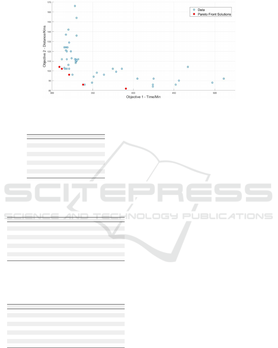
Figure 2: Pareto front and dominated solutions.
Table 3: Information of the locations of each patient (Q
i
for
i = 1, . . . , nl).
Locations Patients
B 1, 2, 3, 5, 6, 7, 13, 15, 16, 19, 20
P 9
A 11, 12
Sm 14
E 4
Rd 8, 10
Sd 17, 18
Mo 21
Ml 22
Table 4 shows the travel times, in minutes, be-
tween locations (H).
Table 4: Time matrix between each location in minutes (H).
A B E Ml Mo P Rd Sm Sd
A 15 16 25 21 18 29 18 15 30
B 16 15 17 18 16 29 15 15 29
E 25 17 15 34 25 37 24 25 37
Ml 21 18 34 15 23 36 27 21 36
Mo 18 16 25 23 15 15 16 15 18
P 29 29 37 36 15 15 25 36 31
Rd 18 15 24 27 16 25 15 15 25
Sm 15 15 25 21 15 36 15 15 26
Sd 30 29 37 36 18 31 25 26 15
Consequently, Table 5 is also presented, with the
distances between locations in kilometers (D).
Table 5: Distance matrix between each location in kilome-
ters (D).
A B E Ml Mo P Rd Sm Sd
A 10 14 24 21 16 28 14 11 33
B 14 10 16 21 19 31 15 11 36
E 24 16 10 35 25 36 21 20 42
Ml 21 21 35 10 30 30 28 22 47
Mo 16 19 25 30 10 12 12 12 21
P 28 31 36 30 12 10 19 24 23
Rd 14 15 21 28 12 19 10 14 25
Sm 11 11 20 22 12 24 14 10 10
Sd 33 36 42 47 21 23 25 10 10
Based on all the data presented, the main objective
is to obtain optimal vehicles scheduling solutions in
order to minimize the total time (in minutes) and the
distance (in kilometers) required to carry out the trips,
the treatments and to return to the starting point.
4.2 Discussion
For this case study, simulations were carried out on a
PC Intel(R) Core(TM) i7 CPU 2.2 GHz with 6.0GB of
RAM. The optimization framework was implemented
in MatLab
R
(MATLAB, 2015).
The values of the control parameters used in GA
for this problem were tuned after preliminary expe-
riments. A population size of 30 individuals (N
pop
=
30) and a probability rate of 50% for crossover and
mutation procedures was used. The stopping crite-
rion was based on the maximum number of iterations
defined as 100 (NI = 100) or the maximum number
of function evaluations of 5000 (NFE = 5000). Since
GA is a stochastic algorithm, 10 runs were carried out
with random initial populations.
The value of the reference point was an ap-
proximation to the ideal vector and the weights
for the objectives varied in the set (w
1
, w
2
) ∈
{(1, 0), (0.75, 0.25), (0.5, 0.5), (0.25, 0.75), (0, 1)}.
For each of the weight vectors, the execution in
MatLab
R
(MATLAB, 2015) was performed.
The multi-objective optimization framework al-
lowed to identify a set of non-dominated solutions,
crucial to provide to the decision maker through the
visualization of solutions in the objective space.
Figure 2 shows the the set of Pareto optimal so-
lutions, i.e. the non-dominated solutions (represented
by a red circle), as well as the dominated solutions
(represented by a blue circle). The position of these
solutions express the trade-offs between the objec-
tives (time in minutes in the x axis and distance in
kilometers in the y axis). It can be seen from Figure 2
that five non-dominated solutions were found, repre-
senting the set of most interesting solutions. There-
fore, these are the solutions that must be taken into
account, because they are optimal in terms of the ob-
jectives, and each solution exhibits the trade-off that
ICORES 2019 - 8th International Conference on Operations Research and Enterprise Systems
440

should be explored. However, it is also important to
analyze the solution in the decision variable space.
In order to illustrate the solutions found in the de-
cision space, Gantt charts are used. Thus, the Gantt
chart aims to represent the vehicle schedule of a so-
lution. In this sense, three different vehicle sched-
ules are presented for home visits, referring to three
non-dominated solutions. The three selected non-
dominated solutions refer to the extreme points in
terms of each of the objectives and the closest solution
to the ideal vector. First, the non-dominated solution
related to the best solution in terms of minimizing the
distance traveled in kilometers (one extreme of Pareto
front) is presented in Figure 3.
Vehicles
Vehicle 1
Vehicle 2
Vehicle 3
Vehicle 4
Patients
1 20 15
11 12
13
10 9
8
17
18
#P
Time traveling
Treatment time
Return to HUB
Objective 1 – Time
Objective 2 – Distance
7
2
Vehicle 5
5
6 19 3
21
14
22 16
4
391
82
Figure 3: Non-dominated solution that minimizes distance.
The scheduling of vehicles for home visits of this
solution shows that the goal of minimizing the dis-
tance presented the solution of 82 kilometers. In turn,
guarantees the visit to all patients but in return a max-
imum of 391 minutes is required.
A further scheduling is also presented for the best
solution in terms of minimizing the time spent in min-
utes (the opposite extreme of the Pareto front). Figure
4 shows the scheduling for this solution.
Vehicles
Vehicle 1
Vehicle 2
Vehicle 3
Vehicle 4
Patients
22 3 2
17 9
18
10 7
16
21
8
Objective 1 – Time
Objective 2 – Distance
14
20
Vehicle 5
6
5 19 13
11 12
309
104
15
1
4
#P
Time traveling
Treatment time
Return to HUB
Figure 4: Non-dominated solution that best represents the
objective of minimizing time.
In this solution, the scheduling presents a signif-
icant improvement of time when compared with the
first solution (309 minutes). However, the day of vis-
its ends with a maximum distance of 104 kilometers.
The scheduling of an intermediate solution to the
two extremes presented above (often referred to as the
“elbow” solution), is illustrated in Figure 5.
Vehicles
Vehicle 1
Vehicle 2
Vehicle 3
Vehicle 4
Patients
6 7 19
4 13
12
11 9
8
18
17
Objective 1 – Time
Objective 2 –
Distance
21
14
Vehicle 5
1
5 15 20
2 22
321
96
10
16
3
#P
Time traveling
Treatment time
Return to HUB
Figure 5: Solution that characterizes the ”elbow” of non-
dominated solutions.
The “elbow” solution has a maximum time of 321
minutes and a maximum of 96 kilometers, since this
is the solution that is closest to the ideal solution.
In summary, a gain in the time spent is achieved
in the ”elbow” solution at the expense of an increase
in the distance traveled when compared to the 1st ex-
treme. However, this decision must be made by the
decision maker taking into account factors such as in-
dividual or mutual preferences, benefits and trade-offs
to derive daily HHC schedules.
In conclusion, the analysis of viable alternatives
gives new valuable information to the decision maker.
Moreover, the multi-objective approach provides al-
ternative optimal solutions that are essential to sup-
port the decision maker to choose adequate schedules
for home visits in a Health Unit.
5 CONCLUSIONS
Home visits at the Health Unit are usually planned
manually and without any computational support,
which implies that, in addition to being a complex and
time-consuming process, the solution obtained may
not be the best. Thus, in an attempt to optimize the
process it is necessary to use strategies that allow to
minimize certain objectives, without, however, wor-
sening the quality of services provided and, always,
looking for the best optimization of the scheduling.
Thus, a multi-objective optimization model was
developed to simultaneously minimize two conflic-
ting objectives: the time spent and the distance trav-
eled (which consequently affects the costs). The
multi-objective optimization problem is scalarized
A Multi-objective Approach to the Optimization of Home Care Visits Scheduling
441

applying the Tchebycheff method and solved by a Ge-
netic algorithm. Different compromise solutions are
obtained. An efficient and fast routine to compute the
non-dominated solutions is implemented. This deci-
sion support system was applied to a case study with
real data.
The optimal alternatives found were analyzed
both in terms of objective functions and decision vari-
ables values. For the decision maker the extreme and
“elbow” solutions can be particularly interesting and
therefore may be carefully investigated. In addition,
the approach allows the possibility of replicating the
problem with different instances, without incurring
additional costs or deficiencies in the service, thus
continuing to be able to serve as a support system,
which today does not yet exist.
As future work perspectives, it is intended to im-
prove the efficiency of the the optimization algorithm,
as well as the model by the inclusion of new objec-
tives and constraints.
ACKNOWLEDGEMENTS
This work has been supported by COMPETE:
POCI-01-0145-FEDER-007043 and FCT - Fundac¸
˜
ao
para a Ci
ˆ
encia e Tecnologia within the project
UID/CEC/00319/2013.
REFERENCES
Allaoua, H., Borne, S., L
´
etocart, L., and Calvo, R. W.
(2013). A matheuristic approach for solving a home
health care problem. Electronic Notes in Discrete
Mathematics, 41:471–478.
Alves, F., Pereira, A. I., Fernandes, A., and Leit
˜
ao, P.
(2018). Optimization of home care visits schedule
by genetic algorithm. In International Conference on
Bioinspired Methods and Their Applications, pages 1–
12. Springer.
Baker, B. M. and Ayechew, M. (2003). A genetic algorithm
for the vehicle routing problem. Computers & Opera-
tions Research, 30(5):787–800.
Benzarti, E., Sahin, E., and Dallery, Y. (2010). A literature
review on operations management based models de-
veloped for hhc services. In European Conference of
Operational Research Applied to Health Care, Gen-
ova, Italy, pages 1–21.
Benzarti, E., Sahin, E., and Dallery, Y. (2013). Operations
management applied to home care services: Analysis
of the districting problem. Decision Support Systems,
55(2):587–598.
Braekers, K., Hartl, R. F., Parragh, S. N., and Tricoire, F.
(2016). A bi-objective home care scheduling prob-
lem: Analyzing the trade-off between costs and client
inconvenience. European Journal of Operational Re-
search, 248(2):428–443.
Bredstr
¨
om, D. and R
¨
onnqvist, M. (2008). Combined vehi-
cle routing and scheduling with temporal precedence
and synchronization constraints. European journal of
operational research, 191(1):19–31.
Deb, K. (2014). Multi-objective optimization. In Search
methodologies, pages 403–449. Springer.
Fikar, C. and Hirsch, P. (2017). Home health care routing
and scheduling: A review. Computers & Operations
Research, 77:86–95.
Gayraud, F., Deroussi, L., Grangeon, N., and Norre, S.
(2013). A new mathematical formulation for the home
health care problem. Procedia Technology, 9:1041–
1047.
Ghaheri, A., Shoar, S., Naderan, M., and Hoseini, S. S.
(2015). The applications of genetic algorithms in
medicine. Oman medical journal, 30(6):406.
Holland, J. H. (1992). Adaptation in natural and artificial
systems: an introductory analysis with applications to
biology, control, and artificial intelligence. MIT press.
Koeleman, P. M., Bhulai, S., and van Meersbergen, M.
(2012). Optimal patient and personnel scheduling
policies for care-at-home service facilities. European
Journal of Operational Research, 219(3):557–563.
MATLAB (2015). version 8.6.0 (R2015b). The MathWorks
Inc., Natick, Massachusetts.
Miettinen, K. (2012). Nonlinear multiobjective optimiza-
tion, volume 12. Springer Science & Business Media.
Nguyen, T. V. L. and Montemanni, R. (2013). Scheduling
and routing in home health care service. In Society 40
th Anniversary Workshop–FORS40, page 52.
Nickel, S., Schr
¨
oder, M., and Steeg, J. (2012). Mid-term
and short-term planning support for home health care
services. European Journal of Operational Research,
219(3):574–587.
Ombuki, B., Ross, B. J., and Hanshar, F. (2006). Multi-
objective genetic algorithms for vehicle routing prob-
lem with time windows. Applied Intelligence,
24(1):17–30.
Pasia, J. M., Doerner, K. F., Hartl, R. F., and Reimann, M.
(2007). A population-based local search for solving
a bi-objective vehicle routing problem. In European
conference on Evolutionary computation in combina-
torial optimization, pages 166–175. Springer.
Rasmussen, M. S., Justesen, T., Dohn, A., and Larsen, J.
(2012). The home care crew scheduling problem:
Preference-based visit clustering and temporal depen-
dencies. European Journal of Operational Research,
219(3):598–610.
Toth, P. and Vigo, D. (2014). Vehicle routing: problems,
methods, and applications. SIAM.
Yalc¸ındag, S., Matta, A., and Sahin, E. (2011). Human re-
source scheduling and routing problem in home health
care context: a literature review. ORAHS/Cardiff,
United Kingdom.
ICORES 2019 - 8th International Conference on Operations Research and Enterprise Systems
442
