Unsupervised Learning of Scene Categories on the Lunar Surface

Thorsten Wilhelm

, Rene Grzeszick

, Gernot A. Fink

and Christian W

ohler

Image Analysis Group, Department of Electrical Engineering, TU Dortmund University, 44227 Dortmund, Germany

Pattern Recognition in Embedded Systems Group, Department of Computer Science, TU Dortmund Universtiy,

44227 Dortmund, Germany

Keywords:

Remote Sensing, Scene Detection, CNN, Unsupervised Learning.

Abstract:

Learning scene categories is a challenging task due to the high diversity of images. State-of-the-art methods

are typically trained in a fully supervised manner, requiring manual labeling effort. In some cases, however,

these manual labels are not available. In this work, an example of completely unlabeled scene images, where

labels are hardly obtainable, is presented: orbital images of the lunar surface. A novel method that exploits

feature representations derived from a CNN trained on a different data source is presented. These features are

adapted to the lunar surface in an unsupervised manner, allowing for learning scene categories and detecting

regions of interest. The experiments show that meaningful representatives and scene categories can be derived

in a fully unsupervised fashion.

1 INTRODUCTION

Unsupervised learning of scene categories is a chal-

lenging and worthwhile task. The advantage of unsu-

pervised learning is easily at hand. The necessity of

annotations is eliminated, which vastly reduces the

human effort necessary to reach a meaningful divi-

sion of the analyzed image data. In this work it will

be shown, that it is possible to achieve a meaningful

categorization by entirely relying on unsupervised le-

arning algorithms.

A large amount of publicly available image data,

which was previously not analyzed with respect to

scene categorization, are satellite images of the lunar

surface. These images can be seen as a special form

of natural scene images. The Lunar Reconnaissance

Orbiter (LRO) is a satellite orbiting the moon since

2009 with the objective to analyze the lunar surface

with various scientiﬁc instruments, including laser al-

timeters and cameras. The quest of the LRO is di-

verse and includes ﬁnding possible landing sites, and

constructing high resolution maps of the moon. The

data are publicly available and hosted by the Natio-

nal Aeronautics and Space Administration (NASA).

In detail, we use the data provided by the Wide Angle

Camera (WAC) global mosaic described in (Speyerer

et al., 2011), which has a spatial resolution of 100

meters per pixel and covers the complete surface of

the Moon, to look for repeating scenes on the lunar

surface. A possible set of scenes is depicted in Fi-

gure 1 with typical scenes being plains, mountains,

highlands, valleys and craters.

Annotations of the lunar surface are scarce and

restricted to the most prominent features like craters

with a large diameter, or the large plains of the near-

side of the moon called lunar mare. It is therefore

hardly possible to use state-of-the-art image classi-

ﬁcation approaches like Convolutional Neural Net-

works (CNNs) which are typically trained in a fully

supervised manner.

One option in such cases is to employ crowd sour-

cing in order to obtain scene or object annotations

(Patterson and Hays, 2012; Perona, 2010). This re-

quires a large number of human annotators and dis-

tributes the annotation effort. In contrast, unsuper-

vised scene learning tries to reveal information wit-

hout the need for annotations. As a result, this task

becomes challenging, especially due to the diversity

of scene images typically requiring top-down know-

ledge. It is usually achieved by either a pure clus-

tering approach with handcrafted features like GIST

(Oliva and Torralba, 2001) or HoG (Dalal and Triggs,

2005). Deep Learning approaches apply Deep Belief

Networks (DBN) (Lee et al., 2009) in which several

Restricted Boltzmann Machines (RBM) are stacked.

The network is then trained by Contrastive Diver-

gence (CD), which is comparable to gradient descent

(Lee et al., 2009).

Another challenge is that in contrast to SAR ima-

ges of terrestrial surface, the number of information

614

Wilhelm, T., Grzeszick, R., Fink, G. and Wöhler, C.

Unsupervised Learning of Scene Categories on the Lunar Surface.

DOI: 10.5220/0007569506140621

In Proceedings of the 14th International Joint Conference on Computer Vision, Imaging and Computer Graphics Theory and Applications (VISIGRAPP 2019), pages 614-621

ISBN: 978-989-758-354-4

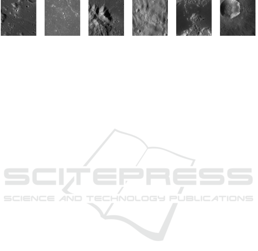
(a) Escarpments (b) Plains (c) Mountains (d) Highlands (e) Valleys (f) Crater

Figure 1: Examples of possible scene categories on the lunar surface extracted from LROC WAC global mosaic (Speyerer

et al., 2011). The range varies from valleys to mountains to more Moon speciﬁc scenes like the crater heavy plains. Each

image depicts an area of roughly 920km

of the lunar surface.

cues is limited (H

ansch, 2014) to grey level intensi-

ties. Furthermore, due to the low resolution of the

WAC images, the number of pixels that is available

for context is also limited.

Leveraging the capabilities of CNNs, a novel met-

hod which combines the strength of pre-trained net-

works with unsupervised learning is proposed. The

method is able to transfer the feature representation

obtained from pre-trained convolution kernels of a

CNN to the novel lunar data, which is then used to

derive object-like detectors and ﬁnally group the ob-

ject appearances into meaningful scene categories.

2 METHOD

For recognizing different scenes on the lunar surface,

it is desirable to have a very descriptive feature repre-

sentation for a given patch p on the surface. State-of-

the-art feature representations can be obtained using

CNNs. However, as labeled data is hardly available,

learning a feature representation using a CNN is not

possible. On the other hand it is also very difﬁcult

to design a meaningful handcrafted feature represen-

tation. In the following it will be shown how to le-

verage learned feature representations from a CNN

trained on a different data source for unsupervised

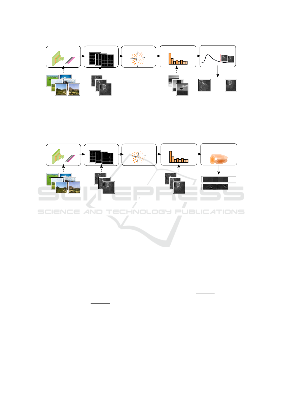
learning. An overview of an unsupervised detector

and scene learning approach are shown in Fig. 2 and

Fig. 3, respectively. From an intermediate layer of

the CNN a feature representation for yet unknown pa-

tches of the lunar surface is derived. Similar to the

Bag-of-Features principle these patches are then clus-

tered in an unsupervised manner using spherical k-

means clustering. This yields a set of representatives

that can be found on the lunar surface, but may as

well occur on any image (e.g. simple edges). For the

detection, a set of negative samples is used in order

to compute the distribution of the representatives on

arbitrary images. Choosing a quantile of least occur-

ring representatives, a set of representatives that is

most discriminative for the lunar surface is chosen.

These representatives are then used as candidates for

detecting different types of lunar surface, e.g. craters

or mountains. For the scene learning, the occurren-

ces of the representatives are clustered again on scene

level, yielding a set of similar scenes. Furthermore,

both scene and detection representatives can be anno-

tated by a human user in order to train a detector or

typical scenes with minimal annotation effort.

2.1 Feature Representation

The VGG16 CNN architecture is used as a basis for

generating the feature representation (Simonyan and

Zisserman, 2014). The convolution part of the net-

work is designed of stacked 3 × 3 convolution lay-

ers and each two convolution layers are followed by a

2 × 2 max pooling layer. Hence, the context is enlar-

ged by two pixels or multiplied by two in the layers

respectively. For example, the context of the ﬁrst two

convolution layers is 3 × 3 and 5 × 5 pixels. The next

step is a max pooling procedure yielding a context of

10 × 10 pixels. Hence, after ﬁve stages of convolu-

tion and pooling layers a context of more than 200

pixels is obtained. For recognition tasks, the convo-

lution part is then followed by fully connected layers.

As the resolution of the images is low, the patch size

that can be used for context is also limited and infor-

mation must be obtained within a context of much less

pixels. Here, the activations of a learned convolution

ﬁlter are chosen as the feature representation for the

patch m (cf. (Razavian et al., 2014)). The convolution

layer can be chosen according to a desired size for the

patch m.

A huge advantage of these off-the-shelf features

is that such a representation can be pre-trained on a

separate dataset (i.e., ImageNet (Deng et al., 2009)).

Given the assumption that the training set contains a

large variability at least a subset may be of interest

for the task at hand. In the following, a new set of

representatives will be learned based on the feature

representation derived from the convolution layer.

Unsupervised Learning of Scene Categories on the Lunar Surface

615

CNN Training

Patch Repr.

Representatives

for Detection

Quantization

Labeled

Training Set

Lunar

Surface Data

Clustering Outlier

Negative

Image Set

...

Figure 2: Overview of the proposed detection method. A Convolutional Neural Network is trained on a labeled dataset (i.e.,

ImageNet (Deng et al., 2009)). From an intermediate layer of the Network a feature representation for yet unknown patches

of the lunar surface is computed. Similar to the Bag-of-Features principle these patches are then clustered in an unsupervised

manner. Then a set of negative samples is used in order to compute the distribution of these cluster centroids on arbitrary

images. Choosing a quantile of least occurring representatives, a set of representatives that is most discriminative for the lunar

surface is chosen. These representatives can then be chosen for detection.

CNN Training

Patch Repr.

Scenes

Quantization

Labeled

Training Set

Lunar Surface Data

Clustering

...

Multinomial

Mixture Model

...

Figure 3: Overview of the scene learning. As for the detection, a CNN is trained on a labeled dataset and features are derived

from an intermediate layer. Clustering these features and quantizing the representation at every pixel in an image then given a

new representation for an image, as is done for image classiﬁcation in Bag-of-Features approaches. These are then clustered

on scene level using a multinomial mixture model in order to obtain different sets of scenes.

2.2 Unsupervised Learning of Filter

Masks

Following the Bag-of-Features principle (Csurka

et al., 2004) the activation of the different convoluti-

ons are clustered in order to obtain a new representa-

tion in an unsupervised manner. A set of patches m

m is

randomly drawn and the activations are derived from

the CNN. As the distribution of the activation does

not necessarily follow those of an Euclidean space,

the cosine distance (Baeza-Yates et al., 1999)

d(i, j)

cos

= 1 −

· f

|| f

|||| f

(1)

is known to work well, where f

and f

are the fe-

ature representations for patch i and j. Spherical

k-means clustering is employed to the data (Zhong,

2005), computing a set of centroids c

c. The centroids

of the clustering process yield a combination of the le-

arned ﬁlters from the pre-trained ﬁlter masks that des-

cribe the new dataset of patches from the lunar surface

well.

The next step is to ﬁnd those representatives that

are especially descriptive for the lunar surface and not

just arbitrary images. Hence, a set of negative image

is chosen. For these images a set of negative fe-

atures n

n is computed at each possible location in the

image. Hence, a large number of negative patches is

computed. All patches are assigned to the set of cen-

troids c

c by hard quantization:

argmin

1 −

· c

||n

||||c

∀ j (2)

This gives a distribution over all centroids. From

these a quantile γ is chosen as the most discrimina-

tive patch representations.

2.3 Detection

After a set of ﬁlter masks is determined, detection

is carried out by computing the Pearson product-

VISAPP 2019 - 14th International Conference on Computer Vision Theory and Applications

616

1019

136

5 1

5 6

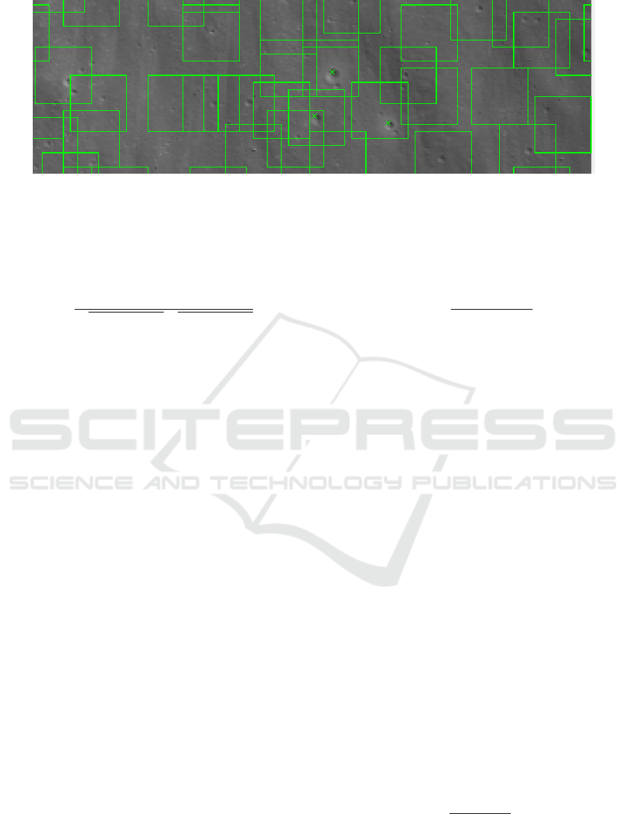
Figure 4: Subset of the detections on the NAC dataset used for crater evaluation. Ground truth crater positions are marked

by a green cross. Detections of the crater ﬁlter are shown by green bounding boxes. The ﬁlter number is noted inside the

bounding boxes for comparison. Note how ﬁlter eight frequently detects small craters, which are not marked by the ground

truth.

moment correlation coefﬁcient r (Fisher, 1915). For

two datasets x and y with n samples r is computed by

∑

i=1

− ¯x)(y

− ¯y)

∑

i=1

− ¯x)

∑

i=1

− ¯y)

. (3)

The correlation coefﬁcient offers the advantage of

a low computational burden even for large datasets,

and is independent of linear transformations, which

makes the detection robust against possibly occurring

linear transformations.

We assume that a ﬁlter detects something in an

image if the corresponding correlation coefﬁcient be-

tween the image representation and the ﬁlters at any

given position surpasses a certain threshold θ

, which

may be set globally or individually for every ﬁlter.

Non maximum suppression (NMS) (Felzenszwalb

et al., 2010) is used to reduce the amount of overlap-

ping detections, which naturally occur around basins

of attractions in the image. Due to the unsupervised

nature of the training process, similar ﬁlter masks may

have a high correlation coefﬁcient at similar locations

in the image. By using NMS we restrict ourselves

to those ﬁlter masks with the highest detection conﬁ-

dence in a speciﬁc region. The amount of overlap can

be adjusted by a threshold θ

nms

2.4 Unsupervised Scene Learning

Based on the detections we try to derive an underlying

scene, which can be interpreted as a latent variable.

Therefore, histograms of the detections are computed

for every image I

. The feature representation of the

images is the same as described in Section 2.1. Ba-

sed on the histograms of the detections a Multinomial

Mixture Model (MMM) with a ﬁxed number of com-

ponents is used to model different object distributions

among different images.

The multinomial distribution has the probability

density function (pdf) (Murphy, 2012, p. 35)

(x;p) ∼



∑

i=1

+ 1



∏

i=1

Γ(x

+ 1)

∏

i=1

, (4)

where d indicates the dimension of the distribution, Γ

the Gamma function, p a vector of probabilities and

the observed counts x. The resulting mixture model

is then

p(X|Θ

Θ) =

∏

i=1

(X;θ

), (5)

with C as the number of components and the elements

π are the corresponding mixture weights. The para-

meters of the whole model are summarized in a set of

parameters Θ.

The model will be estimated in a Bayesian

fashion, so that the mixture weights and the latent pa-

rameters z indicating the class memberships of every

datum are given appropriate probability distributions

as well. We assume that the mixture of latent varia-

bles z follows a categorical distribution with

p(z;π

π) =

∏

i=1

, (6)

and the mixture weights π

π are given by a Dirichlet

distribution, because it is the conjugate distribution

(Raiffa, 1974) to a categorical distribution. This me-

ans that the posterior distribution is given in analy-

tical form and there is no need for computationally

demanding posterior inferences for this variable. The

dirichlet distribution has the pdf

p(π

π;α

α) =

Γ(

∑

i=1

)

∏

i=1

Γ(α

)

∏

i=1

−1

, (7)

with the hyperparameter α

α controlling the shape of

the distribution, which may be used to model the prior

Unsupervised Learning of Scene Categories on the Lunar Surface

617

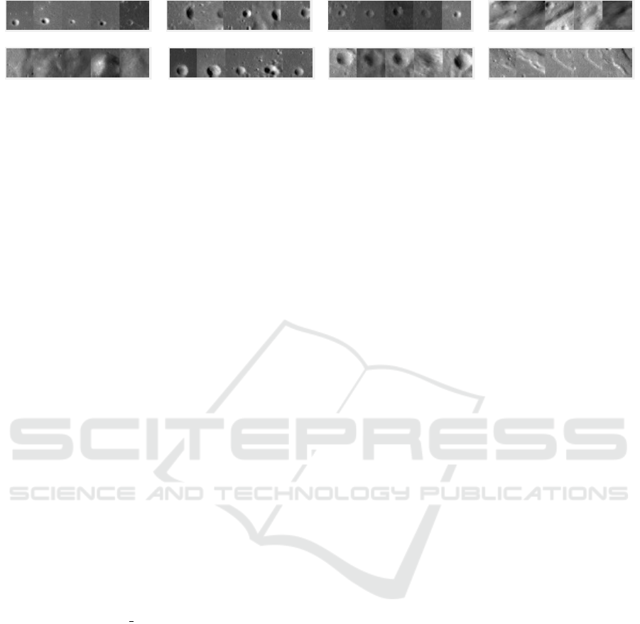
Figure 5: Visualization of the ﬁve nearest neighbors according to the cosine similarity for some of the computed centroids.

The range changes from craters of varying shape and position to pure plains and hill-like structures.

knowledge available about the mixture weights. Note

the analytical similarity to Eq. 6, due to the conjugate

nature of the distributions. Further, the probabilities

of every multinomial M

are given a Dirichlet prior

for the same reason. To estimate Θ we use Markov

Chain Monte Carlo (MCMC) with conjugate poste-

rior updates (Congdon, 2014).

3 EVALUATION

The presented approach has been evaluated on a set

of images of the lunar surface to derive a meaning-

ful scene representation. Note that only a very rough

ground truth describing the properties of the surface

is available. For example, the most prominent craters

have been annotated or some of the larger mountains.

To give some idea of how accurate the derived ﬁlter

masks are, we evaluated the detections on an entirely

different dataset, where annotations for some craters

are available. This is described in Section 3.2. In the

following we describe some details of the implemen-

tation.

3.1 Implementation Details

For the clustering process 400 randomly drawn pat-

ches are extracted from each positive image I

. The

patch size is set to 32 × 32 pixels and the ﬁlter re-

sponse from the conv3 2 layer of the VGG16 net cen-

tered at the patch is used for generating the feature

representation of the patch.

The set of negative images I

is generated based

on the 15 Scenes dataset (Lazebnik et al., 2006). The

dataset has been chosen as it shows arbitrary scenes

and greyscale images, which is an important property

of the lunar surface images. All images in the dataset

have been used as negative samples.

A set of 500 representatives c

c has been used in the

clustering process. A subset of these is depicted in

Fig. 5, where the ﬁve image patches with the lowest

cosine distance are presented. It can be seen that the

variation of typical lunar elements is captured well by

the learned centroids.

3.2 Detection

To evaluate the accuracy of the learned ﬁlter masks an

annotated ground truth will be used. Since the avai-

lability of possible annotations is scarce, we restrict

ourselves to evaluate the accuracy of the most promi-

nent feature on the lunar surface, craters. In detail, we

use annotations provided by (Fisher, 2014) in which

craters with diameters varying from 5 to 41 meters

are marked. The spatial resolution of the analyzed or-

bital images areas amounts to 0.5 meters per pixel,

the excerpts are part of Narrow Angle Camera (NAC)

(Chin et al., 2007) image M126961088LE. The ana-

lyzed region is an area around the crater Hell Q which

has a diameter of 4 km and is among lunar scientists

an interesting ﬁeld for the study of secondary impact

craters, which need to be considered when estimating

the age of a surface area based on crater counts (Fis-

her, 2014).

Note that our approach alleviates the necessity to

include the light direction, the surface albedo, or any

other information apart from the grayscale image into

the detection process. Therefore the detection is more

robust with respect to different illumination conditi-

ons on the planetary surface and can readily be app-

lied to similar problems on different planetary surfa-

ces. Illumination changes are a frequent issue occur-

ring in conjunction with orbital images, because the

data are usually acquired in a bush-broom manner,

where different areas of the planet are scanned in dif-

ferent time steps, during which the position towards

the sun naturally changes.

Further, the ﬁlter masks are trained on the enti-

rely different WAC global mosaic which has a redu-

ced spatial resolution of roughly 100 meters per pixel.

However, we assume that craters appear on every pos-

sible scale on the surface and yet remain comparable

across different scales. Of course, this poses anot-

her challenge for the learned ﬁlter masks apart from

the possible change in illumination with respect to the

training data.

Table 1 provides a summary of the detection re-

sults. Additionally, the same experiments have been

done with patches of the greyscale image data as fea-

tures. While the true positive rate is encouraging, the

false positive rate seems unusually high. The reason

VISAPP 2019 - 14th International Conference on Computer Vision Theory and Applications

618

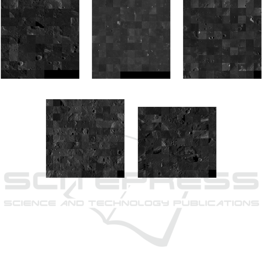
(a) Big structures scene (b) Lunar mare scene (c) Lunar mare with distinctive featu-

res scene

(d) Farside with distinctive features

scene

(e) Farside scene

Figure 6: Visualization of the derived categorization based on the object detections assuming that ﬁve different scenes are

present in the analyzed data. The resulting scene categories meaningfully divide the data in lunar mare and lunar highland

scenes. A further distinction between these two scenes is made by differentiating between the presence and absence of

distinctive lunar features like large craters, mountains, valleys, or the number of small craters present in the scene.

for this behavior is that our algorithm is not able to

distinguish between craters below or above a certain

threshold, but detects every possible crater-like struc-

ture which is similar to a centroid. In Fig. 4 a subset

of the analyzed area is depicted. It is worth noting

that all ground truth positions are covered by a boun-

ding box. While this explains the good recognition

results, the reason for the high false positive rate is

evident as well. A large number of craters, especially

the smallest ones, are not comprised by the ground

truth. However, our algorithm detects a vast majority

of the them as well. In (Fisher, 2014) it is stated that

only craters with a diameter ranging from 5 m to 41 m

are marked. Obviously, our algorithm detects craters

with a diameter less than 5 m.

3.3 Scene Learning

Apart from craters, other characteristic scenes are

prominent on the lunar surface. This includes ridges,

escarpments, crater chains, mountains, valleys, lunar

mare, or lunar highlands. An overview is depicted in

Fig. 1.

Our second goal was to show that it is possible to

derive meaningful scenes in an unsupervised manner

based on the object detections of the previous section.

The mixture model described in Section 2.4 is used

to achieve this goal. The idea is that every scene has

a unique distribution over objects which are present

in the image. A lunar mare scene would for instance

have a high probability of exhibiting small craters and

plain area patches. In contrast, a scene from the far

side of the Moon would have a high probability at fe-

atures which describe a rough surface and small pro-

babilities on the plain area features.

To stress our uncertainty regarding the mixture

weights, we choose to set every entry of the hyper-

parameter α

α to one, and do the same for the prior on

p, the feature probabilities of every multinomial. The

mixture weights π

π, the latent variables z indicating

the class membership, and the p

are estimated with

MCMC. The resulting scene categorization is shown

Unsupervised Learning of Scene Categories on the Lunar Surface

619

Table 1: Evaluation of the crater classiﬁer for various thresholds θ

used to compute the correlation coefﬁcient between every

datum and every centroid c

. True positive rate (TPR), false positive rate (FPR), false negative rate (FNR), and speciﬁcity

(SPC) are presented. Besides the results with CNN features, results for the same analysis with greyscale values as features

(Px) are presented as a baseline for comparison. Best values are marked in bold. The relatively high false positive rate of the

CNN is due to the fact that craters smaller than 5 m are not comprised by the ground truth.

TPR FPR FNR SPC

CNN Px CNN Px CNN Px CNN Px P N

0.65 0.962 0.202 0.032 0.004 0.038 0.798 0.968 0.996 890 1143 750

0.70 0.923 0.140 0.028 0.003 0.078 0.860 0.972 0.997 890 1143 750

0.75 0.836 0.096 0.021 0.002 0.164 0.905 0.979 0.998 890 1143 750

0.80 0.570 0.054 0.010 0.001 0.430 0.946 0.990 0.999 890 1143 750

0.85 0.136 0.012 0.005 0.001 0.864 0.981 0.995 0.999 890 1143 750

in Fig. 6. However, annotations are too scarce to eva-

luate the accuracy. Therefore we restrict ourselves to

a visual inspection.

The found categorization can be divided into two

major categories, lunar mare and highland. While the

former is most dominant in Fig. 6b, the latter is sum-

marized in Fig. 6e. The MMM further derived a scene

which summarizes the boundary between lunar mare

and lunar highland and is depicted in Fig. 6c. This ﬁne

distinction is worth noting and underlines the success

of the presented approach. The remaining scenes des-

cribe either large structures, like ridges or parts of big-

ger craters, or contain scenes where the far side of the

Moon is shown with distinctive features.

4 CONCLUSION

A novel approach towards unsupervised scene lear-

ning has been described. Based on a pre-trained CNN,

state-of-the-art feature representations are adapted to

images of the lunar surface. The resulting feature

representations have been clustered with spherical

k-means in a Bag-of-Features approach to extract

object-like detectors capturing frequently occurring

patterns in the dataset. The accuracy of a subset of

the detectors is evaluated on an annotated dataset of

craters on the lunar surface. Based on the learned ob-

ject detections a scene representation is learned in a

Bayesian fashion. The resulting categorization mea-

ningfully divides the analyzed data into typical lunar

scenes, like lunar mare, lunar highlands, and the bor-

der regions between both.

ACKNOWLEDGMENT

The annotation data of the Hell Q region were provi-

ded by Kurt Fisher. This work has been funded by the

Deutsche Forschungsgemeinschaft (DFG, German

Research Foundation) – Projekt number 269661170.

REFERENCES

Baeza-Yates, R., Ribeiro-Neto, B., et al. (1999). Modern

information retrieval, volume 463. ACM press New

York.

Chin, G., Brylow, S., Foote, M., Garvin, J., Kasper, J., Kel-

ler, J., Litvak, M., Mitrofanov, I., Paige, D., Raney, K.,

et al. (2007). Lunar reconnaissance orbiter overview:

The instrument suite and mission. Space Science Re-

views, 129(4):391–419.

Congdon, P. (2014). Bayesian statistical modelling, volume

704. John Wiley & Sons.

Csurka, G., Dance, C., Fan, L., Willamowski, J., and

Bray, C. (2004). Visual categorization with bags of

keypoints. In Workshop on statistical learning in com-

puter vision, ECCV, volume 1, pages 1–2. Prague.

Dalal, N. and Triggs, B. (2005). Histograms of oriented

gradients for human detection. In IEEE Conference

on Computer Vision and Pattern Recognition (CVPR),

volume 1, pages 886–893. IEEE.

Deng, J., Dong, W., Socher, R., Li, L.-J., Li, K., and Fei-Fei,

L. (2009). Imagenet: A large-scale hierarchical image

database. In Computer Vision and Pattern Recogni-

tion, 2009. CVPR 2009. IEEE Conference on, pages

248–255. IEEE.

Felzenszwalb, P. F., Girshick, R. B., McAllester, D., and

Ramanan, D. (2010). Object detection with discrimi-

natively trained part-based models. IEEE Transacti-

ons on Pattern Analysis and Machine Intelligence,

32(9):1627–1645.

Fisher, K. (2014). An age for hell q from small diameter

craters. In Lunar and Planetary Science Conference,

volume 45, page 1421.

Fisher, R. A. (1915). Frequency distribution of the values

of the correlation coefﬁents in samples from an inde-

ﬁnitely large popu;ation. Biometrika, 10(4):507–521.

ansch, R. (2014). Generic object categorization in PolSAR

images-and beyond. PhD thesis, TU Berlin.

Lazebnik, S., Schmid, C., and Ponce, J. (2006). Beyond

bags of features: Spatial pyramid matching for recog-

VISAPP 2019 - 14th International Conference on Computer Vision Theory and Applications

620

nizing natural scene categories. In IEEE Conference

on Computer Vision and Pattern Recognition (CVPR),

volume 2, pages 2169–2178.

Lee, H., Grosse, R., Ranganath, R., and Ng, A. Y. (2009).

Convolutional deep belief networks for scalable unsu-

pervised learning of hierarchical representations. In

Proceedings of the 26th Annual International Confe-

rence on Machine Learning, pages 609–616. ACM.

Murphy, K. P. (2012). Machine Learning: A Probabilistic

Perspective. The MIT Press.

Oliva, A. and Torralba, A. (2001). Modeling the shape

of the scene: A holistic representation of the spatial

envelope. International journal of computer vision,

42(3):145–175.

Patterson, G. and Hays, J. (2012). Sun attribute database:

Discovering, annotating, and recognizing scene attri-

butes. In IEEE Conference on Computer Vision and

Pattern Recognition (CVPR).

Perona, P. (2010). Vision of a Visipedia. Proceedings of the

IEEE, 98(8):1526–1534.

Raiffa, H. (1974). Applied statistical decision theory.

Razavian, A., Azizpour, H., Sullivan, J., and Carlsson, S.

(2014). CNN features off-the-shelf: an astounding ba-

seline for recognition. In IEEE Conference on Compu-

ter Vision and Pattern Recognition Workshops, pages

806–813.

Simonyan, K. and Zisserman, A. (2014). Very deep con-

volutional networks for large-scale image recognition.

CoRR, abs/1409.1556.

Speyerer, E., Robinson, M., Denevi, B., et al. (2011). Lunar

reconnaissance orbiter camera global morphological

map of the moon. In Lunar and Planetary Science

Conference, volume 42, page 2387.

Zhong, S. (2005). Efﬁcient online spherical k-means cluste-

ring. In IEEE International Joint Conference on Neu-

ral Networks (IJCNN), volume 5, pages 3180–3185.

IEEE.

Unsupervised Learning of Scene Categories on the Lunar Surface

621