Collaborative Merging of Radio SLAM Maps in View of Crowd-sourced
Data Acquisition and Big Data
Kenneth Batstone
a
, Magnus Oskarsson and Kalle
˚
Astrom
b
Centre of Mathematical Sciences, Lund University, S
¨
olvegatan 18A, 222 10 Lund, Sweden
Keywords:
Toa Self-calibration, Crowdsourced, Big Data, Radio Slam.
Abstract:
Indoor localization and navigation is a much researched and difficult problem. The best solutions, usually
use expensive specialized equipment and/or prior calibration of some form. To the average person with smart
or Internet-Of-Things devices, these solutions are not feasible, particularly in large scales. With hardware
advancements making Ultra-Wideband devices more accurate and low powered, this unlocks the potential
of having such devices in commonplace around factories and homes, enabling an alternative method of nav-
igation. Therefore, indoor anchor calibration becomes a key problem in order to implement these devices
efficiently and effectively. In this paper, we present a method to fuse radio SLAM (also known as Time-Of-
Arrival self-calibration) maps together in a linear way. In doing so we are then able to collaboratively calibrate
the anchor positions in 3D to native precision of the devices. Furthermore, we introduce an automatic scheme
to determine which of the maps are best to use to further improve the anchor calibration and its robustness
but also show which maps could be discarded. Additionally, when a map is fused in a linear way, it is a very
computationally cheap process and produces a reasonable map which is required to push for crowd-sourced
data acquisition.
1 INTRODUCTION
Navigation has become a key part of modern civili-
sation, with most people using systems such as GPS
on a daily basis, in their cars or on their person, inte-
grated into their smart phones. The demand for posi-
tioning systems is also increasing with the era of 5G
upon us. With 5G, we expect to see an increase of po-
sitioning accuracy in addition to having more devices,
such as Internet-Of-Things (IoT), to also required po-
sitioning. For example, items in warehouses will re-
quire positioning to enable automation in the ware-
houses to improve efficiency.
Currently GPS provides good positioning for most
users in an outdoor environment. Unfortunately, this
cannot be said once inside a building. Once inside,
the GPS signals are heavily attenuated, meaning the
accuracy of the positioning can decrease to encom-
pass a whole build or more. When this occurs users
must use an alternative system to navigate indoors.
There are currently many options to overcome
this problem but they all come with their own draw-
a
https://orcid.org/0000-0001-8328-1052
b
https://orcid.org/0000-0002-8689-7810
backs. In robotics, many use optical devices to per-
form SLAM (Simultaneous localization and mapping,
(Durrant-Whyte and Bailey, 2006)) such as cameras
and LIDAR, which produce good results but such de-
vices can be expensive and computationally tasking.
This restricts such methods to small environments
with a low amount of dynamic features. For mobile
phone users, a large focus has been using the sig-
nal strength of Wi-Fi networks to perform positioning
since the infrastructure currently exists in most build-
ings but due to the nature of radio signals in complex
environments, they have a low accuracy and with dis-
tance, the errors increase exponentially, (Li et al., ).
One such technology which is commercially
available is Ultra-Wideband (UWB). These devices
are low powered and perform 2-way timing in order
to obtain high precision in positioning, between two
devices. This unlocks the potential of having such de-
vices in common place around factories and homes,
enabling an alternative method of navigation indoors
for people and Internet of Things (IoT) devices.
Another technology which shows promise is
round-trip time (RTT) being enabled on Wi-Fi. With
RTT, it is expected to perform ranging between
routers and mobile device with as low as 1 metre ac-
Batstone, K., Oskarsson, M. and Åstrom, K.
Collaborative Merging of Radio SLAM Maps in View of Crowd-sourced Data Acquisition and Big Data.
DOI: 10.5220/0007574408070813
In Proceedings of the 8th International Conference on Pattern Recognition Applications and Methods (ICPRAM 2019), pages 807-813
ISBN: 978-989-758-351-3
Copyright
c
 2019 by SCITEPRESS – Science and Technology Publications, Lda. All rights reserved
807

curacy. Many modern routers have the ability to per-
form this but currently awaits a firmware update. This
technology uses the 802.11mc IEEE standard, which
has been enabled on Android Pie devices. A strong
advantage to this option is that the infrastructure al-
ready exists.
With these developments comes further issues.
Due to the large number of devices, calibration of
the anchors becomes problematic. Currently large
datasets require vast amounts of memory and process-
ing power, which is impossible for most machines. In
this paper we present new research on methods for
large scale anchor self-calibration problem. Here we
present a method to merge maps together in a linear
way. In doing so we build a library of tools in or-
der to determine the quality of each map and then
to be able to fuse them together to produce a global
map. Additionally, when a map is merged in such a
way, it is a relatively computationally cheap process
and produces a reasonable map which is required to
push for crowd-sourced data acquisition. The pro-
posed method will help bridge the memory require-
ment issues and the ability to select the best datasets.
The proposed method was tested on both simu-
lated and real UWB distance measurements. These
datasets are created using 2-way timing, therefore it
is a Time-Of-Arrival (TOA) self-calibration problem.
The TOA self-calibration problem, is the problem
of determining the positions of a number of receivers
and transmitters given only receiver-transmitter dis-
tances. Here, there is no prior knowledge of the an-
chor positions.
2 BACKGROUND
To solve such problems, one method is to solve a min-
imal case and extend that solution. Minimal cases for
low rank matrix factorization, for missing data, were
investigated in (Jiang et al., 2015). In (Batstone et al.,
2016) a RANSAC paradigm was used in conjunction
with minimal solvers and explored in order to obtain
a robust and fast solution of the TOA self-calibration
problem, with missing data and noise. In (Batstone
et al., 2017) a sequential merging scheme was created
to explore the potential of real-time anchor calibra-
tion. One pitfall of the described scheme was that
as more data was collected, memory requirements
and computational complexity increased which lim-
ited the system.
The TOA self-calibration problem and other in-
door SLAM methods are rarely performed in large
scale using radio. Computer vision research has ad-
dress some issues common to both optical SLAM and
TOA self-calibration problem, such as memory lim-
its, accuracy and computational power. In (Byr
¨
od
and
˚
Astr
¨
om, 2009) and (Byr
¨
od and
˚
Astr
¨
om, 2010),
the authors exploit the structure of the Jacobian so
that memory limits and computational complexity are
improved to allow for SLAM in larger environments
with acceptable losses in accuracy.
In (Puyol et al., 2013), a solution was given for
large scale SLAM, with promising memory require-
ments, computational effort and an accuracy of 0.5m
in 2D, but this works differs since the authors use foot
mounted inertial measurement units (IMU) to crowd-
source SLAM maps, which is not as prevalent as radio
infrastructure. In (Chanier et al., 2008) map fusion
was explored for a multi-robot SLAM framework,
but this method was tested on only two maps. More
research has been conducted in this area, (Schmuck
and Chli, 2017; Liu et al., 2016), but still very few
robots and maps are used when merging. In (Van Op-
denbosch et al., 2018), the authors address the is-
sue of large memory requirements needed for Collab-
orative Visual SLAM. Although optical SLAM and
TOA self-calibration share similar solutions to simi-
lar problems, they differ greatly in accuracy and the
type of data. In optical SLAM many other instru-
ments on the robot assist the formation of the solution
and improves the accuracy. This provides a rich and
reliable dataset. For the TOA self-calibration using
radio systems, it is common that there are fewer an-
chor positions than user sender positions. This means
that when merging anchor positions, the sparsity of
the data is a constraint on the solution and prone to
errors due to the accuracy of the ranging.
3 METHOD
We will now describe the basic underlying geome-
try of our problem. Let R
i
, i = 1, . . . , m and S
j
,
j = 1, . . . , n be the spatial coordinates of m receivers
(e.g. Ultra-Wideband anchors) and n transmitters (e.g.
Crazyflie quadcopter), respectively. For measured
time of arrival t
i j
from transmitter R
i
and receiver
S
j
, we have vt
i j
= kR
i
− S
j
k
2
where v is the speed of
measured signals and k.k
2
is the l
2
-norm. The speed v
is assumed to be known and constant. We further as-
sume that we, at each receiver can distinguish which
transmitter j each event is originating from. This can
be done e.g. if the signals are temporally separated or
using different frequencies. We will in the following
work with the distance measurements d
i j
= vt
i j
. It is
quite common that such data contains both missing
data from poor signal communications and outliers
due to inaccuracies of the hardware measurements.
ICPRAM 2019 - 8th International Conference on Pattern Recognition Applications and Methods
808

The TOA calibration problem can then be defined as
follows,
Problem 1. (Time-of-Arrival Self-Calibration) Given
absolute distance measurements
d
i j
= kR
i
− S
j
k
2
+ ε
i, j
, (1)
where the receiver positions are defined as R
i
, i =
1, . . . , m and transmitter positions as S
j
, j = 1, . . . , n.
Here the errors ε
i, j
are assumed to be either inliers,
in which case the errors are small (ε
i, j
∈ N(0, σ)) or
outliers, in which case the measurements are way off.
Here we will use the set W for the indices (i, j)
corresponding to the inlier measurements.
The Time-of-Arrival Self-Calibration problem can
be solved by computing the bundle adjustment of (2),
shown below.
min
R,S
∑
(i, j)∈W
(d
i, j
− ||R
i
− S
j
||
2
)
2
. (2)
For simplification, (2) can be represented as,
argmin
∑
|d − f (R, S)|
2
(3)
where f (R, S) = ||R −S||
2
can be the nonlinear func-
tion for all combinatins of R, S . Therefore it can be
assumed that there exists an optimal R
?
and S
?
, such
that a
opt
is the minima, ie.
a
opt
=
∑
|d − f (R
?
, S
?
)|
2
. (4)
Then the sum of the residuals can be linearized around
R
?
and S
?
as
a(R, S) ≈ a
opt
+ J

R − R
?
S − S
?

, (5)
where J is the jacobian of f wrt. R and S. The prob-
lem can be reformulated as
a(R, S) ≈ a
opt
+

J
R
J
S


∆R
∆S

. (6)
We can include the contribution of S into the expres-
sion by solving
min
∆S
|a
opt
+ J
R
∆R + J
S
∆S|
2
(7)
which has the closed form solution ∆S =
−(J
T
S
J
S
)
−1
J
T
S
J
R
∆R where
T
denotes matrix trans-
pose. Insertion into (6) yields
a(R, S) ≈ a
opt
+ (I − J
S
(J
T
S
J
S
)
−1
J
T
S
)J
R
∆R, (8)
where I denotes the identity matrix of proper size. In
order to reduce the amount of data being saved in a
database, a matrix A is introduced such that
A = (I − J
S
(J
T
S
J
S
)
−1
J
T
S
)J
R
. (9)
Now A above can be decomposed into A = VU where
U is a upper triangular matrix and V is a unitary ma-
trix. Hence,
|a(R, S)|
2
=|V
T
a(R, S)|
2
≈ |V
T
a
opt
+U∆R|
2
=|a
opt
|
2
+ |U∆R|
2
.
(10)
If two such solutions are available, then the sum of
the norms can be formulated as
|a
1
(R, S)|
2
+ |a
2
(R, S)|
2
≈ |a
1,opt
|
2
+ ...
... + |U
1
(R − R
?
1
)|
2
+ |a
2,opt
|
2
+ |U
2
(R − R
?
2
)|
2
.
(11)
This expression can be minimized for R as
R
opt
= (U
T
1
U
1
+U
T
2
U
2
)
−1
(U
T
1
U
1
R
?
1
+U
T
2
U
2
R
?
2
).
(12)
Which has the general expression, for k maps as,
R
opt
=(U
T
1
U
1
+U
T
2
U
2
+ ... +U
T
k
U
k
)
−1
(U
T
1
U
1
R
?
1
+U
T
2
U
2
R
?
2
+ ... +U
T
k
U
k
R
?
k
).
(13)
Since in reality, some of the calculated maps will
be erroneous due to the environment in which the
measurements are taken, a weighting term is therefore
introduced, where λ
k
∈ [0, 1].
R
opt
(λ) = (λ
2
1
U
T
1
U
1
+ λ
2
2
U
T
2
U
2
+ ... + λ
2
k
U
T
k
U
k
)
−1
(λ
2
1
U
T
1
U
1
R
?
1
+ λ
2
2
U
T
2
U
2
R
?
2
+ ... + λ
2
k
U
T
k
U
k
R
?
k
).
(14)
In order to solve for the problem in (14), a new
variant of the objective function for the full bundle
adjustment (2) is used. Here, one only needs to solve
for the vector λ = [λ
1
, ..., λ
k
] as shown in (15),
min
λ
∑
k
∑
(i
k
, j
k
)∈
˜
W
k
(λ
k
(d
i
k
, j
k
− ||R
opt
i
k
(λ) − S
j
k
||
2
))
2
.
(15)
This, therefore, can be seen as a relaxation of (2),
where the λ variable is similar to the weights in a
weighted optimization. Due to the non-linearity of the
problem, a good initialization is also needed for (15).
To achieve this, a RANSAC scheme was devised to
provide a good initialization but also an indication of
which dataset are best to use, see Algorithm 1.
In this scheme, some of the values are arbitrary
and can be tuned depending on the data type etc.
These values are the 5 random maps and the selec-
tion of all maps within 1m of RMSE distance of the
optimal anchor positions. The reason 5 maps were
chosen is to maintain robustness, since the quality of
maps vary, by choosing 5 maps the optimization can
quickly determine a valid optimal anchor position for
the majority of the iterations. The selection radius
was chosen as generous catchment zone for the in-
lier set, this can be tuned to the specific need of the
datasets.
Collaborative Merging of Radio SLAM Maps in View of Crowd-sourced Data Acquisition and Big Data
809

Algorithm 1: Our RANSAC Merging Scheme.
1: Select 5 random maps
2: Calculate the optimal anchor positions using our merg-
ing algorithm.
3: If: The score of the objective function is the lowest
value so far, select all maps within a 1m of RMSE
distance of the optimal anchor positions. The initial
5 maps keep their λ values from the optimization, all
other inliers are given a value of 0.5 and outliers are
given a value of 0.
4: Repeat steps 1-3 200 times
5: Recalculate a new optimal anchor position using our
merging algorithm with best lambda values as an initial
guess to the optimization.
4 EXPERIMENTAL SETUP
4.1 Simulated Datasets
In order to test our method, three experiments were
devised. The first experiment was to create 40 anchor
positions and 1000 sender positions, randomly to span
a 20×20×20m space. From there the distance matrix
was calculated and Gaussian noise was added with a
variance of 0.18m to simulate UWB measurements.
A full bundle adjustment was then performed, in or-
der to give a comparison to current state of the art
method, (Batstone et al., 2016). The distance matrix,
d, was then divided into 50 equal parts of 40 anchor
positions and 20 sender positions and a map was cre-
ated for each set. Then for each of the 50 maps, our
method was tested with different optimization meth-
ods. Firstly our linear method (13), secondly our lin-
ear method with a weighting factor (14) and lastly a
bundle adjustment. This was then repeated 400 times.
The second experiment was to perform the same
experiment as above but to falsify 30% and 60% of the
50 maps. For the specific percentage of the maps, the
anchor positions were randomly perturbed in a 40cm
radius. The anchor positions were then transformed
to ensure that the first anchor is the origin of the coor-
dinate system and the second anchor on the x-axis and
so on. This transformation was also performed on the
sender positions. This therefore, would give a realis-
tic poor result for those maps. The RANSAC method
was then tested on these datasets to give an under-
standing of the robustness of the proposed merging
schemes and to show how it could be used to deter-
mine good maps. Again this was repeated 400 times.
The third experiment was to test how the num-
ber of maps affects the time it takes to calculate the
optimal solution. Once again, 40 anchor positions
and 1000 sender positions were used like in the first
experiment to simulate UWB measurements. The
RANSAC method was then used to find a solution
for different number of maps, with the time it took
noted, and the time for a full bundle adjustment was
also noted. This was only iterated once.
4.2 Real Datasets
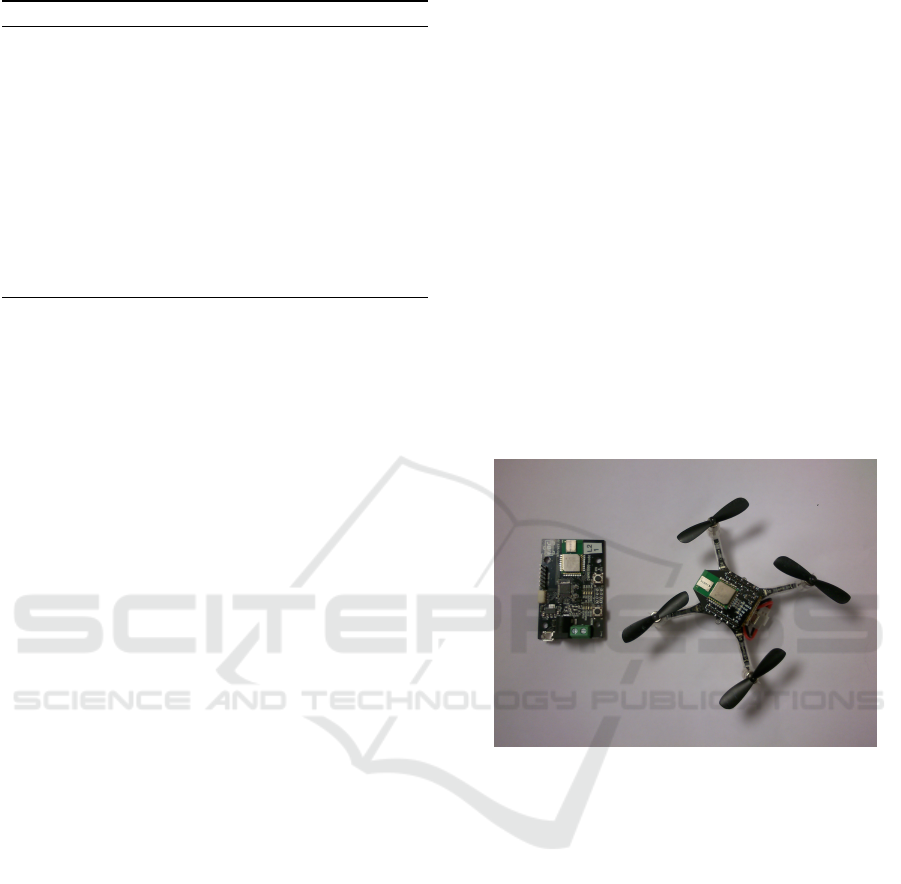
For the final experiment, our algorithms were
tested on real UWB measurements from a Bitcraze,
Crazyflie quadcopter mounted with a UWB device
(Decawave DWM1000 chip) in order to determine if
the proposed method is feasible in a real world situ-
ation, shown in Figure 1. The experiment was con-
ducted in a Motion Capture (MOCAP) Studio to give
ground truth positions to compare our results with.
There were 9 separate datasets with 6 anchors in the
same position for each. The ground truth anchor po-
sitions were calculated using the MOCAP cameras to
a precision of ±1 mm.
Figure 1: Image of the Ultra-Wideband anchor and Bitcraze
Crazyflie quadcopter respectively from left to right.
Distance measurements from the quadcopter to all
the anchors were measured at a frequency of 30 Hz.
The experiments were conducted by moving the
quadcopter, by hand, around the room. The distance
measurements were recorded so that they may be pro-
cessed offline. Our algorithms do not require any
prior knowledge of anchor or quadcopter positions.
The only requirement is that the minimal solver (5,5)
is satisfied for the 3D cases.
5 RESULTS AND ANALYSIS
5.1 Simulated Datasets
In Figures 2 and 3 the results for the first experiment
are shown. For all the experiments the Root Mean-
Squared Errors (RMSE) are a comparison of the cal-
culated optimal anchor positions to the ground truth
ICPRAM 2019 - 8th International Conference on Pattern Recognition Applications and Methods
810

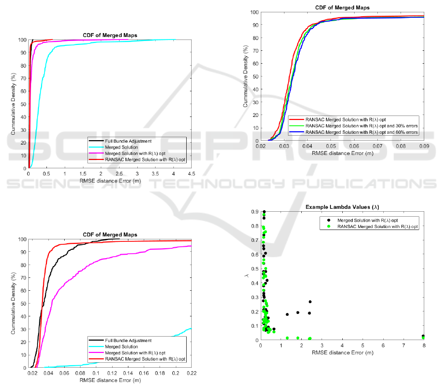
anchor positions. It can been seen that each of the
methods perform differently, with the linear merging
scheme being the least successful. The other three
methods presented show good results since all three
have at least 90% of the solutions with an error under
the UWB distance measurement accuracy of 0.18m,
see Figure 3. The full bundle adjustment result was
expected to be a good solution since the optimization
is minimizing the residual for all 40000 distance mea-
surements. Interestingly, the result for the RANSAC
scheme did not achieve as good as a result for the best
full bundle adjustment solutions but for 55% of the
solutions it did achieve a better result. Furthermore,
it has a steep curve at 0.03m RMSE distance Er-
ror. This indicates that the method reliably produces
a similar result.
Figure 2: This figure illustrates the RMSE error for the each
of the merged maps plotted against its cumulative density
for 400 experiments.
Figure 3: This figure is the same as Figure 2. It illustrates
the RMSE error for the each of the merged maps plotted
against its cumulative density for 400 experiments but only
shows the RMSE range of 0.01 to 0.22.
In Figures 4 and 5, the results for the second ex-
periment are shown. All three solutions show a simi-
lar result, which indicates that by using the RANSAC
scheme it maintains its robustness. This is due to the
RANSAC scheme being able to select a collection
of maps which have similar and good results. This
behaviour is further shown in Figure 5. Figure 5 is
an example of the lambda values obtained after us-
ing the RANSAC scheme and the merging scheme
with lambda optimization. It can be seen that the
RANSAC scheme focuses the optimization of lambda
in one cluster of the maps. This in turn produces bet-
ter optimal anchor positions, the RANSAC scheme
had a RMSE distance error of 0.0379m and the merg-
ing scheme with lambda optimization 0.0498m.
Figure 4: This figure illustrates the RMSE error for the each
of the merged maps with different percentages of errors
plotted against its cumulative density for 400 experiments.
Figure 5: This figure illustrates the RMSE error for each
map plotted against its calculated lambda value.
In Figure 6, the results for the third experiment is
shown. It can be see that the time it takes to find a
solution is dependent on the number of maps. Thus
it also shows that the RANSAC method proposed is
computationally cheaper. In this case, the trend ap-
pears to be parabolic which implies that there is an
Collaborative Merging of Radio SLAM Maps in View of Crowd-sourced Data Acquisition and Big Data
811

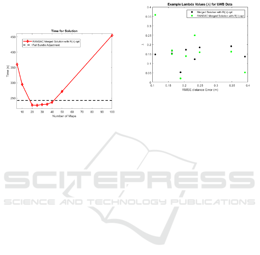
optimal number of maps for each experiment. This
was computed for one random experiment, the times
do vary for each experiment but the trends are similar.
Figure 6: This figure illustrates the computatuional time
for an optimal solution to be found for different number
of maps. The time for a full Bundle Adjustment over all
anchors and senders is also shown as a comparison.
5.2 Real Dataset
In Figure 7 are the lambda values obtained after us-
ing the RANSAC scheme and the merging scheme
with lambda optimization. For this experiment the
RMSE is a comparison of the calculated optimal an-
chor positions to the ground truth anchor positions.
The RANSAC scheme had a RMSE distance error of
0.106m and the merging scheme with lambda opti-
mization 0.1369m. Due to the restricted number of
maps in this case, it is difficult to determine which of
the schemes is better, since nearly all maps are needed
to calculate an optimal map then the lambda value are
similar.
6 CONCLUSIONS
In this paper, a method has been constructed to merge
maps together in a linear way. In doing so we build a
library of tools to determine the quality of each map,
and once the quality of multiple maps were deter-
mined, we can logically merge them together to pro-
duce a global map.
Looking at the results from the MOCAP studio
experiments, in Figure 7 it can be seen, that this
method produces accurate results. For current Ultra-
Wideband systems, the chip sets come with a recom-
mended accuracy of ±0.2m. From our results, we are
also able to achieve this accuracy. It is also interesting
to note that the lambda values for each of the maps are
Figure 7: This figure illustrates the RMSE error for map
plotted against its calculated lambda value. The maps are
created using UWB mounted on a quadcopter.
varied, in particular the map with the smallest error
has a lambda value of ca. 0.35. It shows potentially
that there are not enough separate maps that have been
collected to make a reasonable estimate of the quality
of each map. One would expect the lambda values
to decrease as the RMSE error increases, as seen in
Figure 5, but on this occasions there are erroneous
lambda values. This may be due to the non-linearity
of the self-calibration problem, since there will be
many local minimas, contributions from all maps may
be used.
In the first experiment, our algorithms were
pushed, to test the robustness of the system. From
Figure 2, it can be seen that the anchor positions are
calculated to a high accuracy in comparison to the full
bundle adjustment. It can also be noted that roughly
98% of the merged maps had a RMSE error under
0.25m. Of course, the full bundle adjustment pro-
duces a better result and is considered the gold stan-
dard but in reality it is not a viable option. The bundle
adjustment is very computationally expensive and is
limited by the size of the distance matrix. During the
optimization of the bundle adjustment, it has to esti-
mate 120000 parameters (40 anchors, 1000 senders,
3 degrees of freedom), which modern computers with
large RAM can calculate but any larger wouldn’t be
possible. By partitioning the distance matrix, multi-
ple solutions can be created in parallel, then merged
together. In addition to this, once the lambda values
have been calculated, one would have an estimate of
the quality of each map and the ability to logically
manage each solution with data storage and merged
maps quality in mind. Another benefit, is that the
number of parameters is reduced considerably when
performing the merging algorithm with weights. In
this case from 120000 parameters to 50 parameters.
ICPRAM 2019 - 8th International Conference on Pattern Recognition Applications and Methods
812

The main advantage with such linear fusion is that
it is a relatively computationally cheap process, that
unlocks the potential for crowd-sourced data acquisi-
tion without compromising map quality. In our case,
for the simulated dataset with 60 % errors, to per-
form a bundle adjustment on all 50 maps and merge
them took 47 minutes, whereas the full bundle ad-
justment took 1.5 days on the same machine for all
400 iterations. This can be seen further in Figure
6, with an appropriate number of maps. Although
the computational time reduction can be seen, it is
not as large as the one mentioned for the simulated
dataset with 60 % errors. This may be due to the
the RANSAC initialization, this step produces a ro-
bust and close initialization which reduces the time
needed of our method to converge to the optimal so-
lution. In the case for the simulated data used in ex-
periment 3, since all the maps are viable (no outliers)
then many more maps are initialized with the value
1, hence the computational time is less affected. The
proposed method bridges memory requirement issues
and offers the ability to select the best datasets. In
addition to this, the method would also work for dif-
ferent media type, such as bluetooth, multiple WiFi
frequencies and optical SLAM. Provided that the po-
sitions of the anchor points are the same for each me-
dia.
For future work, the study of a collaborative data
management scheme would be highly advantageous.
In doing so, would give an autonomous way of choos-
ing which parts of the dataset to fuse in order to dis-
card unnecessary data and keep only the required data
to improve a map. For instance, if an office building
were to be mapped using crowd-sourced data, there
would exist areas that would be oversampled, such as
the main entrance and corridors. Whereas a storage
room would be sampled infrequently, therefore an au-
tomatic scheme that would discard the oversampled
areas would be advantageous to data management.
In summary, this would be a way of determining the
uniqueness of a given map.
REFERENCES
Batstone, K., Oskarsson, M., and
˚
Astr
¨
om, K. (2016). Ro-
bust time-of-arrival self calibration and indoor local-
ization using wi-fi round-trip time measurements. In
2016 IEEE International Conference on Communica-
tions Workshops (ICC), pages 26–31.
Batstone, K., Oskarsson, M., and
˚
Astr
¨
om, K. (2017). To-
wards real-time time-of-arrival self-calibration using
ultra-wideband anchors. In 2017 International Con-
ference on Indoor Positioning and Indoor Navigation
(IPIN), pages 1–8.
Byr
¨
od, M. and
˚
Astr
¨
om, K. (2009). Bundle Adjustment us-
ing Conjugate Gradients with Multiscale Precondi-
tioning.
Byr
¨
od, M. and
˚
Astr
¨
om, K. (2010). Conjugate Gradient
Bundle Adjustment, volume 6312, pages 114–127.
Springer.
Chanier, F., Checchin, P., Blanc, C., and Trassoudaine, L.
(2008). Map fusion based on a multi-map slam frame-
work. In 2008 IEEE International Conference on Mul-
tisensor Fusion and Integration for Intelligent Sys-
tems, pages 533–538.
Durrant-Whyte, H. and Bailey, T. (2006). Simultaneous lo-
calization and mapping: part i. IEEE Robotics Au-
tomation Magazine, 13(2):99–110.
Jiang, F., Oskarsson, M., and
˚
Astr
¨
om, K. (2015). On the
minimal problems of low-rank matrix factorization. In
Proc. Conf. Computer Vision and Pattern Recognition.
Li, B., Salter, J., Dempster, A. G., and Rizos, C. In-
door positioning techniques based on wireless lan. In
LAN, First IEEE International Conference on Wire-
less Broadband and Ultra Wideband Communica-
tions, pages 13–16.
Liu, S., Mohta, K., Shen, S., and Kumar, V. (2016). Towards
collaborative mapping and exploration using multiple
micro aerial robots. In Experimental Robotics, pages
865–878. Springer.
Puyol, M. G., Robertson, P., and Angermann, M. (2013).
Managing large-scale mapping and localization for
pedestrians using inertial sensors. In 2013 IEEE In-
ternational Conference on Pervasive Computing and
Communications Workshops (PERCOM Workshops),
pages 121–126.
Schmuck, P. and Chli, M. (2017). Multi-uav collaborative
monocular slam. In 2017 IEEE International Con-
ference on Robotics and Automation (ICRA), pages
3863–3870. IEEE.
Van Opdenbosch, D., Aykut, T., Alt, N., and Steinbach,
E. (2018). Efficient map compression for collabora-
tive visual slam. In 2018 IEEE Winter Conference on
Applications of Computer Vision (WACV), pages 992–
1000. IEEE.
Collaborative Merging of Radio SLAM Maps in View of Crowd-sourced Data Acquisition and Big Data
813