Deep Separable Convolution Neural Network for Illumination

Estimation

Minquan Wang

and Zhaowei Shang

College of Computer Science, Chongqing University, No. 174 Shazheng Street, Chongqing, China

Keywords: Illumination Estimation, Deep Convolution Network, Separable Convolution, Global Average Pooling.

Abstract: Illumination estimation has been studied for a long time. The algorithms to solve the problem can be roughly

divided into two categories: statistical-based and learning-based. Statistical-based algorithm has the advantage

of fast computing speed but low accuracy. Learning-based algorithm improve the estimation accuracy to some

extent, but generally have high computational complexity and storage space. In this paper, a new deep

convolution neural network is proposed. We design the network with more layers (11 convolution layers)

than the existing methods, remove the “skip connection” and “Global Average Pooling” is used to replace

“Fully Connection” layer which is commonly used in the existing methods. We use the separable convolution

instead of the standard convolution to reduce the number of parameters. In reprocessed Color Checker Dataset,

compared with the present state-of-the-art the proposed method reduces the average angular error by about

60%. At the same time, using separable convolution and “Global Average Pooling” reduces the number of

parameters by about 86% compared with do not use them.

1 INTRODUCTION

As we all know, image has three main features: color,

texture, and shape. As a global feature, color feature

describes the surface properties of the image or image

region. However, the extraction of color features

needs to be carried out under standard illumination,

so the estimation of illumination (you also can call it

“color constancy”) in the image becomes the top

priority. Although there has been a long history of

research on illumination estimation, it is far from

achieving the goal of "fast and good", and there are

still many problems in practical application.

Currently, illumination estimation algorithms can

be roughly divided into two types: statistical-based

algorithms and learning-based algorithms. Statistical-

based methods estimate parameters based on the

statistical attributes of the image and some

presuppositions, such as Grey-World (Buchsbaum

and Gershon, 1980), Shades-of-Grey (Finlayson et

al., 2004), Grey-Edge (Joost et al., 2007), White-

Patch (Brainard and Wandell, 1986) and so on. The

common advantage of these algorithms is their low

computational complexity. But these methods require

some illumination estimation experience and do not

work well when the scene is complex. Learning-

based methods build model with image features to

estimate illumination. With the development of

machine learning, some techniques have been applied

to build models, such as Gamut mapping (Gijsenij et

al., 2010), Bayesian (Gehler et al., 2008), SVR (Funt

and Xiong, 2006).

They only reduced the error by about 10%

compared with the statistical algorithm, but the

computational complexity was several times or even

tens of times the original.

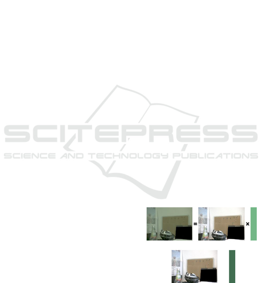
Figure 1: An example of “illumination estimation”: a color-

casted image I equals a color-corrected image W multiply

the illumination L.

I W L

Ours W and L, err = 0.96

Wang, M. and Shang, Z.

Deep Separable Convolution Neural Network for Illumination Estimation.

DOI: 10.5220/0007684308790886

In Proceedings of the 11th International Conference on Agents and Artiﬁcial Intelligence (ICAART 2019), pages 879-886

ISBN: 978-989-758-350-6

879

State-of-the-art methods are associated with

convolutional neural networks (CNN). Thanks to the

strong fitting ability of CNN, remarkable results have

been achieved. Simone Bianco (Bianco S et al., 2017)

designed a network with a convolution layer 、 a

pooling layer and a full connection layer. At the same

time it use a small patch (32x32) as input to reduce

the amount of computation and use the average of

local results as the global results. It got the best results

of the time, and was very fast. Hu Y (Hu et al., 2017)

fine-tuned the Squeeze Net (Iandola et al., 2016) and

use a big patch (512x512) as input, because the bigger

patch size represents more information and use

squeeze module to reduce the number of parameters.

In general, the research and application of

illumination estimation still face two main problems:

first, whether the accuracy of illumination estimation

can be further improved?

Second, whether the storage space and amount of

calculation of the algorithm can be further reduced?

To address these problems, we propose a new

network with deep separable convolution. First, we

use a deeper network structure which has 11

convolution layers to improve the estimation

accuracy. Then, we use separable convolution

(Chollet, 2017) and “Global Average Pooling” (Lin

M et al., 2013) in the network to reduce the number

of network parameters.

In reprocessed Color Checker Dataset (Shi, 2010),

compared to the state-of-the-art algorithm, the mean

angular error has been reduced by about 60%. And

after using separable convolution and “Global

Average Pooling”, the network parameters are

reduced by about 86%. The storage space of our

method is 0.62MB. So it can be easy used in

equipment of “Internet of things” (IoT) or mobile

device.

2 RELATED WORK

2.1 Illumination Estimation

The goal of “illumination estimation” is to dislodge

the illumination in image. According to Lambertian

reflection (Basri, 2001) theory, the color of the image

is determined by both the pixel value of the image and

the illumination. It can be represented by equation, as

in (1).

I W L=

(1)

I represents the real image we got. And W represents

the white-balanced image and L represents RGB

illumination which is shown in Fig. 1.

( )

MAX

E MAX

MAX







(2)

“Illumination estimation” is get the image W from

image I. We should build a model f(I)= L. Then we

can get W = I / L. At first, people used statistical-

based algorithm to build models. White-patch

(Brainard and Wandell, 1986) considered that the

maximum pixel value of the three channels of RGB

reflects the illumination color of the image, as in (2).

MAX(F

) represents the maximum pixel value of

the channel. The advantage of this method is that it is

easy to calculate, but because of its assumption that

all three channels of RGB should have total reflective

surfaces, it is difficult to satisfy in real life. In general,

the effect of this method is poor.

Gray-World (Buchsbaum and Gershon, 1980) is a

method like White-patch. It considered that the

average pixel value of the three channels of RGB

reflects the illumination color of the image, as in (3).

( )

MEAN

E MEAN

MEAN







(3)

Compared with White-patch, this method has the

advantage of low computational cost, but the error of

recovery is larger.

In addition to the two methods mentioned above,

there are many similar statistical-based algorithms,

such as Shades-of-Gray (Finlayson et al., 2004),

Gray-Edge (Van De et al., 2007). Because the data set

in the study had a single light intensity and many of

the parameters in these models is built by experience

and reasonable hypothesis, the result of these models

was poor and they have no extensive applicability.

In recent years, learning-based algorithms have

become popular. Gamut mapping (Gijsenij et al.,

2010) calculates a regular gamut of color. For the

image of unknown light source, the mapping between

the gamut of color and the standard gamut of color is

calculated, and the illumination is obtained. Bayesian

(Gehler et al., 2008) and SVR (Funt and Xiong, 2006)

mode the key features such as brightness and

chromaticity distribution of image pixels to estimate

illumination. NIS (Gijsenij and Gevers, 2011) trains

a maximum likelihood classifier to choose method to

estimate illumination. EB (Joze and Drew, 2014)

trains the model by unsupervised learning a model for

each training surface in training images.

These methods are relatively stable and have a

wide range of applications compared to statistical-

based algorithms, and the results are better.

ICAART 2019 - 11th International Conference on Agents and Artiﬁcial Intelligence

880

Now, convolution neural network has been used

to solve this problem. CCC (Barron, 2015) extracted

the chromaticity histogram of the image as input and

train the model by a small convolution neural

network. Convolution neural network is introduced to

solve the illumination estimation problem for the first

time, and the results are better than before. However,

because of the simplicity of the network, the effect is

not very good. CNN (Bianco et al., 2017) combined

support vector regression with convolution neural

network. This method solves the problem of multiple

illumination, but because of the simplicity of network

structure, it also does not obtain very good results.

Cheng (Cheng et al., 2014) used principal component

analysis to estimate the illumination in spatial

domain. DS-Net (Shi, 2016) trained a two-branch

structure network and chooses an estimate from

among the hypotheses. Oh (Oh, 2017) transformed

illumination estimation into a classification problem.

Fc4 (Hu, 2017) fine-tuned the Squeeze Net (Iandola,

2016) with confidence-weighted pooling and up to

now got the best result. They all get a good result by

using convolution neural network, but some layers

such as “Fully Connection” in these networks lead to

a waste of storage space.

2.2 Separable Convolution

Convolution layer is the core of convolution neural

network. The traditional way of convolution is well

known, and the study of it has never stopped. AlexNet

(Krizhevsky, 2012) used “group convolution” to

reduce the computation of network. ResNet (He,

2016) used “skip connection” to make it possible for

deep networks to be trained. However, these networks

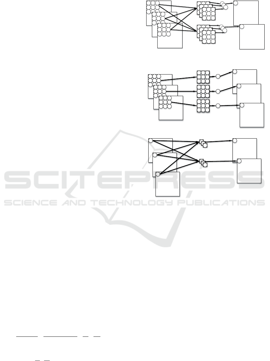
all use standard convolution which is shown in Fig.

2(a).

We can see that the correlation between the

channel and the space of the feature map is considered

at the same time. There is a question why we consider

them at the same time? So, separable convolution

(Chollet, 2017) which is shown in Fig. 2(b) is

designed to solve it. In Fig. 2, we can see that the

number of parameters are reduced about 50% when

use separable convolution.

In (4), there are feature maps which have size

**H W N

and the kernel is

*KK

and the channel of

output is

( )

K M HWN

Separable

conv K MHWN M K

= = +

(4)

In network, the computation of network can be

reduced about

when use separable convolution.

(a) Standard convolution

(b) Separable convolution

Figure 2: The difference between standard convolution and

separable convolution.

2.3 “Global Average Pooling”

In NIN (Network in Network) (Lin, 2013), authors

came up with a lot of interesting ideas. One of them

is the correlation analysis of replacing “Fully

Connection” with “Global Average Pooling”. In the

classification task, we all know that using the “Fully

Connection” layer can improve the network

performance to some extent, but it has a huge

disadvantage that the number of parameters is too

large. Large amount of parameters will lead to a waste

of time and storage space in training and testing, and

there will be over-fitting problem. “Global Average

Pooling” uses the average of features map to replace

them as output. This not only reduces the number of

parameters, but also gives practical meaning to each

channel. The details about “Fully Connection” and

“Global Average Pooling” are shown in Fig. 3.

Input

Kernel

3x3

Feature

maps

Input

Kernel

3x3

Depthwise

feature

Depthwise conv

Depthwise

feature

Kernel

1x1

Pointwise

feature

Pointwise conv

Deep Separable Convolution Neural Network for Illumination Estimation

881

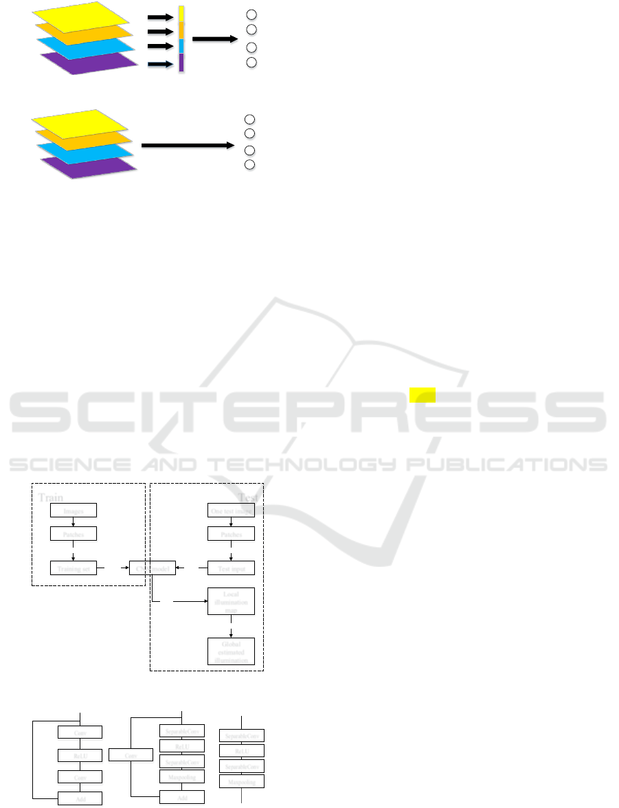
(a) “Fully Connection”

(b) “Global Average Pooling”

Figure 3: The difference between “Fully Connection” and

“Global Average Pooling”.

3 PROPOSED METHOD

In training, we transform all images into patches and

the size of them is 64x64. The label of them is the

same as the label of image which they belong to. Then

we randomly choose 20,000 of them as training set to

train the model.

In testing, test image is transformed into patched

which have the same as training set. And all of them

are put into the model and get a result to build a local

illumination map. Then we get the median of the map

as the estimated illumination of the image. The

procedure is shown in Fig. 4.

Figure 4: The procedure of proposed method.

Figure 5: The difference between our modules.

3.1 Network Structure

3.1.1 Basic Module

We use basic convolution module as the basic unit of

network structure such as ResNet module (He, 2016),

Xecption module (Chollet, 2017). In designing the

structure of module, we refer to the above two

structures. But compared with them, we use separable

convolution instead of standard convolution and

remove “skip connection” from module. Because

“skip connection” not only transmits useful

information, but also becomes the bridge of noise

transmission. And we've proved through experiments

that with skip connection, the effect is very bad. The

corresponding experimental results are shown in

Table 3. Using separable convolution can reduce

number of parameters. The difference between our

modules is shown in Fig. 5. The corresponding

experimental results are shown in Table 4.

3.1.2 Network

We design a convolution neural network which has

11 convolution layer (contain 4 modules). At the

architectural level, we mainly draw on two important

ideas of VGG [24]. The first is to replace the large

convolution kernel with the small convolution kernel.

The second is to increase the number of feature maps

while reducing the size of feature maps. In tiny

networks, it is important to have enough number of

channels to process the information (Zhang, 2017).

Some details of the network structure are shown in

Table 1 and Fig. 6.

In the network, we get a patch with size (64x64x3)

as input. Then we use two standard convolution layers

followed by four basic modules. At the end of

network, we use a standard convolution layer to

change the channel of output into three. We use GAP

(Global Average Pooling) to replace the Flatten and

“Fully Connection” layer.

This kind of network structure design is a result

that we get the best performance after a lot of

experiments. According to the hardware equipment

and the actual pursuit of the effect can be adjusted

appropriately. The corresponding experimental

results are shown in Fig. 7.

3.1.3 Difference from Other Methods of

using CNN

Compared with the other methods of using CNN

(convolution neural network) to solve the

illumination estimation problem the network

structure we designed has the following difference.

Fully

Connection

Outputs

Feature

maps

Flatten

Average

Outputs

Feature

maps

Images

Patches

Training set

Randomly select 20000

CNN model

Training

Test input

Testing

Patches

One test image

Everyone is used

Local

illumination

map

Output

Global

estimated

illumination

Median

Train Test

SeparableConv

ReLU

SeparableConv

Maxpooling

Conv

Add

Conv

ReLU

Conv

Add

SeparableConv

ReLU

SeparableConv

Maxpooling

ResNet Module

Xecption Module

Proposed Module

ICAART 2019 - 11th International Conference on Agents and Artiﬁcial Intelligence

882

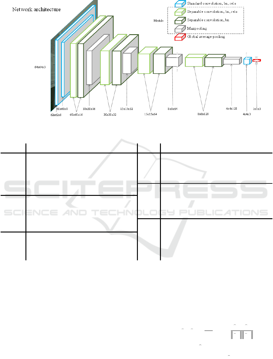
Figure 6: Architecture of our deep separable convolution. We show the different operation by using different color.

Table 1: The details of our network.

Operation

Output

Parameters

Operation

Output

Parameters

Input

64x64 , 3

module

3x3 Separable Conv ,

Bn, Relu

15x15 , 64

2,592

Label

1x1 , 3

3x3 Separable Conv , Bn

15x15 , 64

4,928

layer

3x3 Conv , Bn, Relu

62x62 , 8

248

Maxpooling

8x8 , 64

layer

3x3 Conv , Bn, Relu

60x60 , 8

608

module

3x3 Separable Conv ,

Bn, Relu

8x8 , 128

9,280

module

3x3 Separable

Conv , Bn, Relu

60x60 , 16

264

3x3 Separable Conv , Bn

8x8 , 128

18,048

3x3 Separable

Conv , Bn

60x60 , 16

464

Maxpooling

4x4 , 128

Maxpooling

30x30 , 16

Last

layer

3x3 Conv

4x4 , 3

3,459

module

3x3 Separable

Conv , Bn, Relu

30x30 , 32

784

Output

Global average pooling

1x1 , 3

3x3 Separable

Conv , Bn

30x30 , 32

1,440

Maxpooling

15x15 , 32

Compared with (Barron, 2015) and (Bianco,

2017), a deeper network is designed. Because we

have the experience that more parameters have better

fit ability. And in the same number of parameters, a

“thin and deep” network works well than a “fat and

shallow” network. The reason is a “thin and deep”

network can transform the problem into some small

problems to solve by modules. And we always want

to solve small problems, the network is also.

Compared with (Hu, 2017), the basic module of

network is different and (Hu, 2017) uses transfer

learning to train network. We train the network by

initialization. Of course, another main difference is

the comprehension about building a simple network.

3.2 Loss Function

We train the network by minimizing the loss function

which can be called angular error. The loss function

is shown as in (5). It obtains the angle error between

the real illumination vector and the predicted

illumination vector.

( )

180

, arccos



•









(5)

In the loss function,

represents the normalized

result of the real value and

represents he

normalized result of the output of the network.

Deep Separable Convolution Neural Network for Illumination Estimation

883

Table 2: Compared to the other methods (in degree).

Mean

Med

Tri

Best 25

Worst 25

95% Quant

6.36

6.28

2.33

10.58

11.30

7.55

5.68

6.35

1.45

16.12

4.93

4.01

4.23

1.14

10.23

11.90

5.13

4.44

4.62

2.11

9.26

4.22

2.33

2.91

Bayesian

4.82

3.46

3.88

1.26

10.49

SVR

7.99

6.67

14.61

NIS

4.19

3.13

3.45

1.02

9.22

11.7

2.77

2.24

5.52

Cheng

3.52

2.14

2.47

0.50

8.74

CCC

1.95

1.22

1.38

0.35

4.76

5.85

CNN

2.36

1.98

SqueezeNet-FC

1.65

1.18

1.27

0.38

3.78

4.73

DS-Net

1.93

1.12

1.33

0.31

4.84

5.99

2.16

1.47

1.61

0.37

5.12

DSCNN

0.67

0.49

0.52

0.16

1.52

1.86

4 EXPERIMENTS AND RESULTS

We have done a lot of experiments to verify the

correctness and effectiveness of our method. In

addition to verifying the effect of the method, we also

verify the setting of some super parameters in the

method through experiments.

4.1 Experimental Setting

We built the whole network through the Keras

framework. To train the network, we use Adam

(Kingma, 2014) to minimize the loss function. All of

the parameters are initialized by “glorot_uniform”

(Glorot, 2010), and to prevent overfitting, we add L2

regularization to all convolution parameters. We train

the network for 200 epochs. In the top 50 epoch, we

use a learning rate of 0.001. In 50 to 150 epoch, we

use a learning rate of 0.0001. In the last 50 epoch, we

use a learning rate of 0.00005.

4.2 Datasets

We use the reprocessed Color Checker Dataset (Shi,

2000) for benchmarking. The dataset has 568 images.

These images were got by using two high quality

DSLR cameras (Canon 5D and Canon1D) with all

settings in auto mode. Using the advice of the authors

of the dataset, each image needs to be subtracted from

the black level in order to solve the color constancy

problem. For the Canon 5D the black level is 129 and

for the Canon 1D it is zero. In all images, there is a

Macbeth Color Checker (MCC) to show the ground

truth illumination color. Because it contains a lot of

color information and our network is learning color

features, we set these pixels of MCC to zero.

We cut the original image to a patch with the size

64x64. We randomly selected 20, 000 patches as the

training set. In training, we selected 2/3 of them for

training and the remaining 1/3 for validation. And the

size of batch is 128.

4.3 Evaluation Criterion

We use it as an evaluation criterion by calculating the

angle between the estimated and real value of the

illumination. The same as Hu Y (Hu et al., 2017), we

get the error matrix of the 568 images and report the

following statistics: mean, median, tri-mean of all the

errors, mean of the lowest 25% of errors, mean of the

highest 25% of errors and 95% Quant. 95% Quant

means 95 percent of the errors is smaller than this

value.

4.4 Experiments

4.4.1 Compared to Other Methods

We selected five statistics-based and ten learning-

based algorithms as benchmark algorithms. The

statistics-based algorithms are: Gray-World (GW),

White-Patch (WP), Shades-of-Gray (SG), Gray-Edge

(GE). The learning-based algorithms are: Gamut

Mapping (GM), Bayesian, SVR, Natural-Image-

Statistics (NIS), Exemplar-Based Color Constancy

(EB), Cheng et al., (2014), CCC, CNN, FC4, DS-Net,

Oh. We show the results in Table 2.

The results show that most of the learning-based

ICAART 2019 - 11th International Conference on Agents and Artiﬁcial Intelligence

884

methods are better than those based on statistics,

which proves that the learning-based method can

better extract the color features of images. Moreover,

the proposed method is superior to the current optimal

algorithm in all evaluation indexes. The average error

is reduced by about 60%. There are two reasons why

we are able to make such a huge advance. First,

compared to most of the CNN-based algorithms, in

our algorithm the depth and width of the network are

guaranteed. This makes the network strong enough to

express feature. Second, compared to the algorithm

which have more parameters like Hu Y (Hu et al.,

2017), the selection of our network structure and the

number of parameters is appropriate. And we do not

use transfer learning to train our model. This avoids

the impact of other types of data.

4.4.2 Whether “Skip Connection” Is Used or

Not

In the design of deep convolution neural network,

“skip connection” is a good technique to ensure the

convergence of the network. However, “skip

connection” is not suitable for all tasks. In

illumination estimation, because of the small amount

of data, if “skip connection” is introduced, it will

propagate noise, which is not good for network

training. In Table 3, we experimented with whether to

add “skip connection” and found that the results were

the same as we had expected.

Table 3: Compare between whether use “skip connection”.

Mean error

YES

0.74

0.67

4.4.3 Effects of Some Super Parameters

It is very important to set some super parameters in

convolutional neural networks. If improper super

parameters are selected, the effect of the whole

network may be very poor or the network is difficult

to converge. Therefore, it is more reliable to

determine some of the parameters by experiment than

to select them directly from experience.

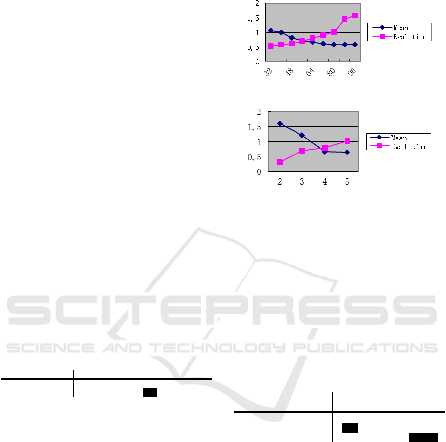
In Fig. 7(a), we can see that when the size of patch

is bigger than 64, there is no significant improvement

in performance. And as we all know, the computation

of neural network is gradual improvement. So, we

choose 64 as our input.

In Fig. 7(b), we can see that when the number of

modules is bigger than 4, there is no significant

improvement in performance. And as we all know,

the computation of neural network is gradual

improvement. So, we choose 4 to build network.

(a) Abscissa axis expresses the size of patch. Vertical axis

expresses the mean angular error and the evaluation time for one

image.

(b) Abscissa axis expresses the number of blocks. Vertical axis

expresses the mean angular error and the evaluation time for one

image. The size of patch is 64. When use five modules, we remove

the pooling layer from the last module.

Figure 7: Results about effects of “size of patch” and

“number of modules”.

4.4.4 Cost of Storage Space

Compared with the current algorithms, we want to get

a better and faster model. So when we design the

network, we change the convolution layer and the

“Fully Connection” layer, which contain a lot of

parameters. We use separable convolution instead of

standard convolution and remove the “Fully

Connection” layer.

Table 4: Cost of storage space.

Mean

error

Conv

layers

Storage

space

SqueezeNet-FC

1.65

35.2MB

Proposed(standard)

0.47

3.56MB

Proposed(separable)

0.67

0.62MB

Because we do not use “Fully Connection” and

less convolution layers, the cost of storage space is

reduced by about 90%. At the same time, using

separable convolution replace standard convolution

can reduce storage space by about 86% at the cost of

error increased from 0.47 to 0.67.

5 CONCLUSIONS

In this paper, we propose a new algorithm to solve the

illumination estimation problem. Due to the shallow

network used in the current convolution neural

network methods, we design a deeper convolutional

Deep Separable Convolution Neural Network for Illumination Estimation

885

neural network and obtain good results. The average

angle error on the reprocessed Color Checker Dataset

is reduced by about 60%. In addition, we use the

separable convolution and “Global Average Pooling”

to reduce the computational complexity of the

network and the storage space of the network by

about 86%. Further improvement of estimation

accuracy and estimation of multi-scale illumination

will be the focus of our future work.

REFERENCES

Shi L. Re-processed version of the gehler color constancy

dataset of 568 images[J]. http://www. cs. sfu. ca/~

colour/data/shi_gehler/, 2000.

Buchsbaum, Gershon. "A spatial processor model for object

colour perception." Journal of the Franklin institute

310.1 (1980): 1-26.

Finlayson, Graham D., and Elisabetta Trezzi. "Shades of

gray and colour constancy." Color and Imaging

Conference. Vol. 2004. No. 1. Society for Imaging

Science and Technology, 2004.

Van De Weijer, Joost, Theo Gevers, and Arjan Gijsenij.

"Edge-based color constancy." IEEE Transactions on

image processing 16.9 (2007): 2207-2214.

Brainard D H , Wandell B A . Analysis of the retinex theory

of color vision.[J]. Journal of the Optical Society of

America A-optics Image Science & Vision, 1986,

3(10):1651-1661.

Gijsenij A , Gevers T , Weijer J V . Generalized Gamut

Mapping using Image Derivative Structures for Color

Constancy[J]. International Journal of Computer

Vision, 2010, 86(2-3):127-139.

Gehler P V, Rother C, Blake A, et al. Bayesian color

constancy revisited[C]// IEEE Conference on Computer

Vision & Pattern Recognition. 2008.

Funt B, Xiong W. Estimating Illumination Chromaticity via

Support Vector Regression[C]// Color & Imaging

Conference. 2006.

Bianco S., Cusano C., Schettini R. Single and Multiple

Illuminant Estimation Using Convolutional Neural

Networks[J]. IEEE Transactions on Image Processing,

2017, 26(9):4347-4362.

Hu Y , Wang B , Lin S . FC^4: Fully Convolutional Color

Constancy with Confidence-Weighted Pooling[C]//

IEEE Conference on Computer Vision & Pattern

Recognition. IEEE Computer Society, 2017.

Iandola F N, Han S, Moskewicz M W, et al. SqueezeNet:

AlexNet-level accuracy with 50x fewer parameters and

<0.5MB Model Size[J]. 2016.

Chollet, François. "Xception: Deep learning with depthwise

separable convolutions." arXiv preprint (2017): 1610-

02357.

Lin M , Chen Q , Yan S . Network In Network[J]. Computer

Science, 2013.

Basri, Ronen, and David Jacobs. "Lambertian reflectance

and linear subspaces." Computer Vision, 2001. ICCV

2001. Proceedings. Eighth IEEE International

Conference on. Vol. 2. IEEE, 2001.

Gijsenij A, Gevers T. Color constancy using natural image

statistics and scene semantics[J]. IEEE Transactions on

Pattern Analysis and Machine Intelligence, 2011,

33(4): 687-698.

Joze H R V, Drew M S. Exemplar-based color constancy

and multiple illumination[J]. IEEE transactions on

pattern analysis and machine intelligence, 2014, 36(5):

860-873.

Barron J T. Convolutional color constancy[C]//

Proceedings of the IEEE International Conference on

Computer Vision. 2015: 379-387.

Bianco S, Cusano C, Schettini R. Single and multiple

illuminant estimation using convolutional neural

networks[J]. IEEE Transactions on Image Processing,

2017, 26(9): 4347-4362.

Cheng D, Prasad D K, Brown M S. Illuminant estimation

for color constancy: why spatial-domain methods work

and the role of the color distribution[J]. JOSA A, 2014,

31(5): 1049-1058.

Shi W, Loy C C, Tang X. Deep specialized network for

illuminant estimation[C]// European Conference on

Computer Vision. Springer, Cham, 2016: 371-387.

Oh S W, Kim S J. Approaching the computational color

constancy as a classification problem through deep

learning[J]. Pattern Recognition, 2017, 61: 405-416.

Krizhevsky A, Sutskever I, Hinton G E. Imagenet

classification with deep convolutional neural

networks[C]// Advances in neural information

processing systems. 2012: 1097-1105.

He K, Zhang X, Ren S, et al. Deep residual learning for

image recognition[C]// Proceedings of the IEEE

conference on computer vision and pattern recognition.

2016: 770-778.

Simonyan K, Zisserman A. Very deep convolutional

networks for large-scale image recognition[J]. arXiv

preprint arXiv:1409.1556, 2014.

Kingma D P, Ba J. Adam: A method for stochastic

optimization[J]. arXiv preprint arXiv:1412.6980, 2014.

Glorot X, Bengio Y. Understanding the difficulty of

training deep feedforward neural networks[C]//

Proceedings of the thirteenth international conference

on artificial intelligence and statistics. 2010: 249-256.

Zhang X , Zhou X , Lin M , et al. ShuffleNet: An Extremely

Efficient Convolutional Neural Network for Mobile

Devices[J]. 2017.

ICAART 2019 - 11th International Conference on Agents and Artiﬁcial Intelligence

886