Technical Validation of the RLS Smart Grid Approach to Increase Power

Grid Capacity without Physical Grid Expansion

Ram

on Christen

, Vincent Layec

, Gwendolin Wilke

and Holger Wache

Department of Computer Science, University of Applied Science Lucerne, Rotkreuz, Switzerland

Institute of Information Systems, University of Applied Science and Arts of Northwestern Switzerland, Olten, Switzerland

Keywords: Smart Grid, Power Grid, Grid Capacity, Grid Reinforcement, Load Prediction, Load Management.

Abstract:

The electriﬁcation of the global energy system and the shift towards distributed power production from sus-

tainable sources triggers an increased network capacity demand at times of high production or consumption.

Existing energy management solutions can help mitigate resulting high costs of large-scale physical grid rein-

forcement, but often interfere in customer processes or restrict free access to the energy market. In a preceding

paper, we proposed the RLS regional load shaping approach as a novel business model and load management

solution in middle voltage grid to resolve this dilemma: market-based incentives for all stakeholders are pro-

vided to allow for ﬂexible loads that are non-critical in customer processes to be allocated to the unused grid

capacity traditionally reserved for N-1 security of supply. We provide a validation of the technical aspects of

the approach, with an evaluation of the day-ahead load forecasting method for industry customers and a load

optimization heuristics. The latter is tested by a simulation run on a scenario of network branch with provoked

capacity bottlenecks. The method handles all provoked critical network capacity situations as expected.

1 INTRODUCTION

With the ongoing change away from fossil resources

toward electric power, an increase in electric power

demand and in production and consumption concur-

rency can be foreseen. As a result, higher grid capac-

ities are required to avoid grid congestion. To help

mitigate the high costs of assumed future large scale

physical grid expansions, IT-based energy manage-

ment solutions in the ”Smart Grid” have been pro-

posed for a more efﬁcient use of existing capacities

(Atzeni, 2014). Yet, most of these grid-optimizing ap-

proaches interfere with customer processes and do not

rely on market-based principles. In contrast, market-

based energy management approaches usually disre-

gard the perspective of grid optimization.

In (Bagemihl et al., 2018), a business model has

been proposed that provides market-based incentives

to all stakeholders on the medium voltage grid lev-

els to utilize so-called ”conditional” ﬂexible loads for

grid capacity optimization. The business model is as-

sociated with a load management approach for ”Re-

gional Load Shaping” (RLS) with a day-ahead opti-

mization heuristics that considers both, customer-side

energy prizes and grid capacity constraints of network

branches, at the same time. In order to allow for grid

capacity increase without necessitating physical grid

expansion, the RLS approach proposes to allocate

for so-called ”conditional loads” the currently unused

grid capacity dedicated to ensuring the (n-1) security

of supply. That capacity is reserved for the case of

rare grid disturbance where one branch takes over the

loads of another branch. I.e., conditional loads com-

prise ﬂexibilities that may be temporarily shedded in

the event of grid disturbance. They contrast with ”un-

conditional loads”, which require security of supply

all-time, such as, loads required for industrial produc-

tion processes.

In the present paper, we test and validate the tech-

nical aspects of the RLS approach, namely the RLS

optimization heuristics and the underlying day-ahead

load forecasting method. For testing and validation

we simulate network congestions by extrapolating

a real world scenario of our pilot customers to fu-

ture scenarios with increased power demand and sup-

ply. We show that the proposed load scheduling so-

lution with its prize optimization heuristics handles

the critical network capacity situations as expected.

For the evaluation of the day-ahead load forecasting

method, we evaluate the Mean Absolute Percentage

Error (MAPE) as a measure of accuracy and show

that the results achieved with our pilot customers’

Christen, R., Layec, V., Wilke, G. and Wache, H.

Technical Validation of the RLS Smart Grid Approach to Increase Power Grid Capacity without Physical Grid Expansion.

DOI: 10.5220/0007717101230130

In Proceedings of the 8th International Conference on Smart Cities and Green ICT Systems (SMARTGREENS 2019), pages 123-130

ISBN: 978-989-758-373-5

123

data sets are comparable with results in the literature.

Additionally, we evaluate the prediction reliability as

a means for the Distribution System Operator (DSO)

and end customer to assess the prediction quality from

a pragmatic perspective.

2 STATE OF THE ART

2.1 Load Scheduling Approaches

Shifting the electrical consumption to another time is

a Demand Response (DR) case, a change in electric

usage by prosumer (household or industrial customer)

from its normal demand pattern in reaction to an in-

centive payment. The review of (Shariatzadeh et al.,

2015) distinguished dispatchable programs where the

prosumers let the DSO control their systems from

non-dispatchable programs where the prosumers de-

centrally set their load schedule. The latter category

spans from simple Time-Of-Use (TOU) with constant

day and night prices to Real-Time Pricing (RTP), a

tariff changing at each time step. In (Doostizadeh and

Ghasemi, 2012), the information about the price is

communicated one day in advance so prosumers do

not need to predict prices. But automatic schedulers

participating with the same information will plan their

load in the same cheapest timestep and unfortunately

create new peaks (Zhao et al., 2013). The formula-

tion of the schedulers (mathematical programming,

metaheuristics or other controllers) depends on the

type of tariff system, but also on the type of elec-

trical loads, their operating constraints, the number

of timesteps, the type of variables (without integer or

not), as classiﬁed in (Shaikh et al., 2014). The case of

photovoltaic in combination with several battery types

is addressed in (Thirugnanam et al., 2018). The is-

sue of synchronisation is tackled in (Mohsenian-Rad

and Leon-Garcia, 2010) with tariff of Inclining Block

Rates (IBR) where high consumption levels are dis-

suasively expensive. (Hunziker et al., 2018) showed

that the total load of a community of prosumers can be

well shaped with tariffs combining RTP with IBR. So

far, no tariff system targets the paradox that in grids

half of the transmission capacity is reserved as a re-

dundancy for the rare case of failure and remains an

expensive unused resource.

2.2 Prediction Methods for Day-ahead

Forecasting for Industry Customers

A growing importance of efﬁcient energy usage and

an even more decentralized sustainable power pro-

duction increases the focus in research on prediction

of time series for power demand. In that ﬁeld, James

W. Taylor has done several works in time series pre-

diction such as (Taylor et al., 2006; Taylor et al., 2007;

Taylor, 2010). A major differentiation in research is

done in the aggregation level of the predicted power

demand. Commonly it is said, the higher the level the

less the prediction accuracy. This behavior is shown

in several papers (Zufferey et al., 2016; Arora and

Taylor, 2016; Mirowski et al., 2014). A comparison

of the aggregation level versus the prediction accu-

racy in (Mirowski et al., 2014) conﬁrms this depen-

dency. A similar behaviour is also shown by Kong et.

al that predicted individual residential power demand

with a Long Short-Term Memory (LSTM) network

and a precision of a MAPE of approx. 44% com-

pared to an aggregate forecast with a MAPE of ap-

prox. 8% (Kong et al., 2017). The strength of a LSTM

network for an electrical load forecast compared to

other common methods such as Support Vector Re-

gression (SVR) are shown in (Zheng et al., 2017) with

an achieved MAPE of less than 6%.

Further, for a prediction also the usage of power

is differentiated, i.e. whether the time series is of a

residential or an industrial consumption. In (Kong

et al., 2017) it is mentioned that industrial electric-

ity consumption patterns would be more regular than

residential ones such that Ryu et al. achieved in (Ryu

et al., 2016) a prediction accuracy for industrial loads

with a MAPE of about 8.85%. Less accurate predic-

tions were obtained in (Ghofrani et al., 2011) for res-

idential loads by means of a Kalman ﬁlter estimator.

Mocanu et. al presented in (Mocanu et al., 2016) dif-

ferent deep learning approaches whereas the imple-

mentation of a Factored Conditional Restricted Bolz-

man Machine (FCRBM) outperformed several Ma-

chine Learning (ML) algorithms.Comparable results

were achieved by Marino et. al by using a LSTM net-

work (Marino et al., 2016) and Shi for household load

forecasting (Shi et al., 2018).

3 THE RLS APPROACH

3.1 Increasing Grid Capacity

In most grids system availability must be guaranteed

in case of failure of a single network component such

as, e.g., a power line or transformer unit. As a result a

percentage of the grid capacity is not used in normal

operation, but reserved for this so-called (N-1) secu-

rity of supply. However, the large majority of days go

without grid failure.

The RLS approach proposes to allocate the nor-

mally unused grid capacity reserved for (N-1) secu-

SMARTGREENS 2019 - 8th International Conference on Smart Cities and Green ICT Systems

124

rity of supply to conditional loads. Here, conditional

loads are loads for which (1) (N-1) security of supply

is not essential, (2) that are highly price-sensitive, and

(3) that are ﬂexible and may thus be used for price

optimization purposes via load management. Condi-

tional loads comprise, e.g., the charging of stationary

batteries for internal consumption or power heat cou-

pling for fuel substitution. Unconditional loads are

all other loads.

Since security of supply is by deﬁnition not es-

sential for conditional loads this unused grid capac-

ity may be dedicated to them without compromising

the important security of supply level for conventional

household and industrial loads: in case of a branch

failure, conditional loads are shedded to provide se-

curity for unconditional loads.

Figure 1 illustrates a simpliﬁed version of the used

and unused grid capacity. Here, the component’s

maximal capacity is split exemplarily in two capac-

ity bands of 50% each. The lower band shown in

blue is the capacity used in normal operation, while

the upper band shown in grey represents the unused

capacity reserved for security. We call this band the

N-1 band because it ensures N-1 security to another

branch. Notice that the width of the N-1 band of a

network branch is determined by the component with

smallest capacity. The day-ahead prediction of un-

conditional loads (dark blue) and the scheduling of

conditional loads (green) is the subject of the rest of

this paper.

Figure 1: Example of a load schedule split in unconditional

loads (blue) and conditional loads (green).

In the RLS approach, the market-based incentive

for customers to register some of their ﬂexibilities as

conditional loads is (1.) a load schedule management

for energy price optimization and (2.) a signiﬁcantly

lower grid fee compared to unconditional loads. In-

centives for distribution system operators (DSO) to

implement the RLS approach comprise (1.) the pos-

sibility to postpone or avoid large scale physical grid

expansion, (2.) achieving a small increase in income

by additionally charged grid costs for the N-1 band,

and (3.) higher transparency within the grid due to

customer side load measurement and DSO-registered

load schedules.

3.2 Scheduling Conditional Loads

The goal of the day-ahead scheduling of conditional

loads is to minimize energy prizes for all customers

connected to the network branch under consideration.

The minimization is subject to (1.) the customers’

chosen prizing models, (2.) to their operating con-

straints (dependent on the ﬂexible loads in use), and

(3.) to given grid constraints. Since regulations re-

quire that grid control and provision of energy supply

must be operated by separate legal entities, the man-

agement software is split in two independent subsys-

tems: the Grid Manager (GM) is operated by the DSO

and monitors grid constraints; the Energy Manager

(EM) implements the customer perspective and col-

lects the individually price-optimized load schedules

of all connected customers and aggregates them. An

iterative optimization heuristics implements the inter-

action of GM and EM in order to ensure grid and cus-

tomer constraints. Each iteration comprises two steps:

1. Local optimization: The EM calculates a price-

optimized conditional load schedule for a partici-

pating customer, which (if given) respects the grid

constraints prescribed by step 2. It submits the

schedule to the GM.

2. Global optimization: The GM aggregates the ac-

cumulated loads from different customers and

checks grid capacity constraints. In case the N-1

band capacity is exceeded, the GM curtails each

customer’s schedule according to their chosen

prizing model and submits to the EM an adapted

schedule based on load optimization on the aggre-

gated level; they then can optimise theri schedule

again (step 1).

The process is reiterated until a predeﬁned time-based

deadline is reached and ﬁnal schedules of the next day

are sent to the controllers of each customer’s devices.

In step one, each customer initially submits his

desired schedule of conditional loads for the next day

to the GM, i.e. a time series of the power of each ag-

gregate a for each timestep t. It is computed by solv-

ing a minimization of the daily energy costs subject

to operations constraints of conditional loads, such as

the energy balance for battery. Costs of substituted

fossil fuels and costs of electricity - via the actual

power and the actual electricity price - are considered.

The actual power is the net power supplied by the

grid, so the sum of unconditional resp. conditional

loads, corrected by the own photovoltaic (PV) pro-

duction. The electricity price is made of a spot price

timeserie predicted for year 2035 plus other fees OF

(grid, taxes and duties). For unconditional loads in

the so-called Standard Tariff (STT), OF is assumed

to grow up to 10 ct. / kWh until 2035. We introduce

Technical Validation of the RLS Smart Grid Approach to Increase Power Grid Capacity without Physical Grid Expansion

125

a so-called Power Alliance Tariff (PAT) with reduced

OF of only 4.8 ct / kWh in order to give a ﬁnancial

incentive to use conditional loads. OF is 0 ct / kWh

when the power is fed back to the grid, so that the use

of own overproduction of PV remains the cheapest

option to schedule conditional loads, whereas import-

ing power at PA Tariff during timesteps of low spot

price becomes the second cheapest option.

In step two, initially submitted schedules are ag-

gregated, controlled and adjusted by the GM. On the

time steps with synchronized original loads exceed-

ing the grid limit, a centralized algorithm computes

an allocation respecting them with consideration of

the load asked by each customer c and their ﬁnan-

cial participation of this system of conditional loads.

Once completed, a decentralized algorithm allocates

loads at customer level for each of the aggregates.

3.3 Day-ahead Load Forecasting

The second technical aspect of the RLS approach

evaluated in the paper is the day-ahead prediction

of the unconditional loads of industry customers. It

serves two purposes: (1.) to provide customers with

higher transparency and thus better control of their

energy usage - it thereby serves as an additional in-

centive to participate in the program; (2.) to allow for

optimized usage of the currently unused grid capacity

in future scenarios.

For the day-ahead load forecasting of customer

load proﬁles, a model selection approach (MSA) has

been chosen. Thereby, a set of different time series

forecasting models are trained, ﬁtted and evaluated

based on historical load proﬁle data that comprises

14, 28, 42, 56 and 70 days for every individual cus-

tomer. The best model and training data length is cho-

sen separately for each customer based on the MAPE

performance evaluation metric. The MSA is executed

in regular time intervals (e.g. every month) in order

to allow for continuous adaptations to changes in the

customer load proﬁle characteristics.

16 different prediction models where included:

As a benchmark model, the load proﬁle of the pre-

vious workday / non-working day was used as fore-

cast for the following day, respectively. The simi-

lar days model was included in three variants: SD1

uses the median of a set of historical days of the same

weekday (e.g., the ﬁve previous Mondays) as a fore-

cast, SD2 uses the median of a set of previous work-

days or non-working days, respectively, and SDEns

takes the median of the forecasts of SD1 and SD2.

The classical time series prediction models Expo-

nential Smoothing (ES), Random Walk Drift (RWD),

Hold Winters (HW), Auto-Regressive Integrated Mov-

ing Average (ARIMA) and Generalized Autoregressive

Conditional Heteroskedasticity (GARCH) each where

applied both directly to the original load proﬁle and

to the residual of the load proﬁle after decomposition.

The latter version is referred to with the add on Dec

after the model name: ES Dec, RWD Dec, HW Dec,

ARIMA Dec, and GARCH Dec. Finally, a support vec-

tor machine with a radial bias kernel was applied in

both variants, SVR and SVR Dec.

4 SCHEDULING VERIFICATION

In order to test the scheduling approach for condi-

tional loads, we provoke a grid congestion in a sce-

nario based on real data of three pilot customers A, B

and C and one ad-hoc customer X.

4.1 Settings of the Experiment

Present energy usage of customers A, B and C are

classiﬁed in Table 1 in thermal or non thermal usage.

Photovoltaic panels will be installed on their roofs.

A new customer X, representative for several new

customers like freight shipping companies with new

Power-To-Gas units up to 7 MW but without signiﬁ-

cant own compulsory loads nor PV, is added to simu-

late a congestion of the band of conditional loads. No

other grid related carrier (district heating) or off grid

(heating oil, pellets, etc.) is considered here. New

units of Table 2 are assumed to be added. ”Other”

aggregates of C (a food industry) are hereby cooling

machines using the frozen food as thermal storage and

substituting electricity of a cooling machine of a later

timestep of the same day.

Table 1: Energy carrier and usage (kW peak) of customers.

usage electric cooling electric process process with gas heat from gas

A 700 1000 - 500

B - 300 - 200

C 2000 1700 1000 1000

Table 2: Assumed new conditional loads and PV (kW).

P-to-Heat P-to-Gas Battery other PV

A 500 - - - 1500

B - 300 100 - 900

C - - - 2x250 1900

X - 7000 - - -

A ﬁctive grid conﬁguration with all customers A,

B, C and X in the same branch is assumed to evaluate

our method. Each power line (asset) has here a capac-

ity of 12 MW and is not used over 6 MW to provide

reserve capacity. In the ﬁrst asset of the branch, com-

pulsory loads reaches today 5.4 MW (no bottleneck).

SMARTGREENS 2019 - 8th International Conference on Smart Cities and Green ICT Systems

126

With the new loads, the sum grows to 13.8 MW (bot-

tleneck). Moreover, simultaneous conditional loads

can reach 8.4 MW and thus exceed the capacity of 6

MW of the N-1 band.

4.2 Initially Submitted Schedules

Figure 2 with power on left y-axis against time on x-

axis shows the initial solution (i.e. before control of

grid limits) of the load scheduling problem for cus-

tomers A (top row), B (middle row) and X (bottom

row) for the cloudy winter day of January, 11th. Con-

sumption respectively production are displayed sepa-

rately on the left resp. right graph. Grey bands repre-

sent the split in Standard Tariff for compulsory loads

in the lower part of positive power and Power Alliance

Tariff in the upper part with conditional load. Nega-

tive power is fed back to the grid. In customer A,

the PV unit (yellow) substitutes part of electricity im-

port from grid (black), and is used to run the power-

to-heat unit (blue) to substitute natural gas. The P-t-

H unit will also run with the cheap electricity price

of PAT (black, brindled) during afternoon hours with

the lowest spot price of the day. The Power-to-Gas

units of Customer X, as well as the Power-to-Gas

unit (blue) and the charging (red) of battery of Cus-

tomer B will run at the same afternoon hours as cus-

tomer A due to the spot price. Discharging (green)

happens here in morning hours, before charging, ei-

ther for substituting import from grid (black) or for

feed back to grid (purple), with a sufﬁcient battery

capacity assumed in this model. The cooling units of

Customer C (not displayed) are modelled like a bat-

tery but with the hygiene constraint that charging can

only precede discharging, as the storage medium is

the frozen food. Therefore they run in the morning at

a different timestep than A and B.

4.3 Curtailment in Case of Excess Load

On Grid Level: GM controls the cumulative load of

all customers, displayed in Figure 3 with compulsory

resp. conditional loads in the lower resp. upper part.

When the lowest electricity spot price is attained be-

tween 2 p.m. and 6 p.m., conditional loads from A,

B and X get aggregated with 7.9 MW (left graph).

The conditional loads exceed the grid capacity limit

of 6 MW of the N-1 band and should be reduced by

1.9 MW. The loads are re-allocated for all customers

A, B and X according to a rationing scheme of Table

3. The curtailment is done proportionally to the num-

ber of points (allowances) of each customer without

exceeding their initially submitted schedule. In case

a customer asked less than its allowance (here C), the

remaining non-allocated capacity is redistributed iter-

atively among the other customers to avoid waste of

capacity.

Table 3: Curtailment on grid level.

points submitted (kW) ﬁnal (kW)

A 500 500 379.7

B 400 400 303.8

C 500 0 0

X 7000 7000 5316.5

sum 8400 7900 6000

On Aggregate Level: After each customer reads

the amount of its curtailment for each timestep, it

computes the local curtailment on the level of each

aggregate. Aggregates are modelled here with an inte-

ger number of stages between a minimal (here 0) and

maximal power. The allocation with least wasted ca-

pacity is solved as a subsum problem. Table 4 shows

the local curtailment of timestep 53 of customer B.

Both units are cut in order to reach 303 kW, the max-

imal value not exceeding the allowance of 303.8 kW

from Table 3. The cases of Customer A (with only one

unit of P-to-H) and of Customer X (with four units of

P-to-G) are treated in a similar way. The schedule

of ”discharging” is ﬁnally adjusted on customers with

battery like B to respect the daily energy balance.

Table 4: Curtailment on aggregate level for customer B.

max levels original (kW) ﬁnal (kW)

P-to-G 300 100 300 204

charging 100 100 100 99

sum 400 - 400 303

4.4 Discussion

With new loads, two issues were expected: (1.) In

the absence of the concept of conditional loads, a grid

reinforcement would have been needed in the ﬁrst as-

set (even with only the new loads of customers A, B

and C). (2.) in presence of customer X and due to load

synchronization at the cheapest timestep, the 6 MW of

N-1 band were overbooked in the initial schedules and

a reinforcement would have been needed in absence

of curtailment. The RLS approach with use of N-1

band and with curtailments solves both problems and

enables ﬁnding schedules valid for both sides. The

schedule curtailed by GM fulﬁlls the grid limit with-

out wasting of capacity in the N-1 band. EM reduces

schedules on aggregate level accordingly without nei-

ther wasting capacity nor disturbing the energy bal-

ance of batteries. In the aggregated schedule in Figure

3, the effective use of the N-1 band drops from 26.7 %

(left) to only 22.0 % (right, after curtailment) but the

system is safe for all stakeholders to be operated.

Technical Validation of the RLS Smart Grid Approach to Increase Power Grid Capacity without Physical Grid Expansion

127

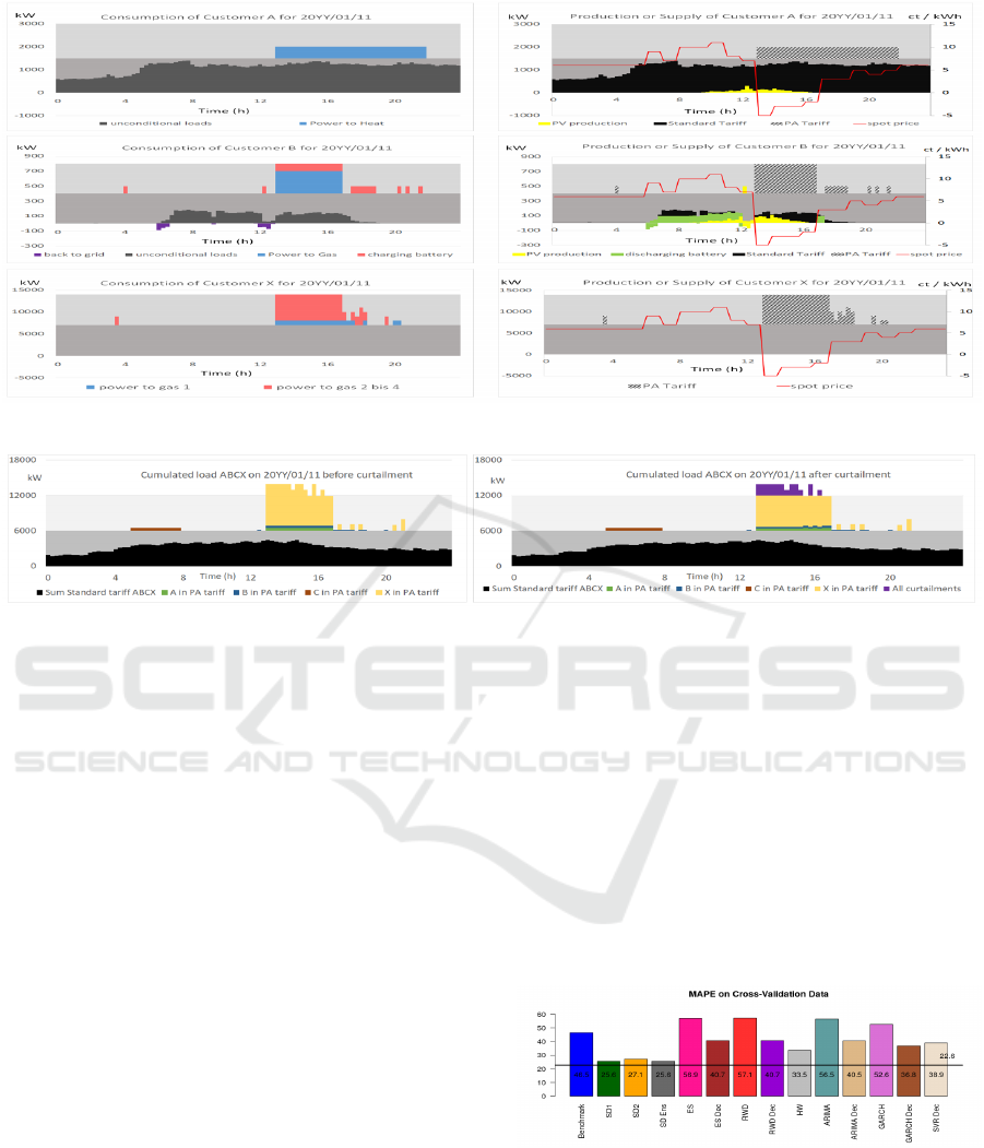
Figure 2: Initial solution of schedule for customers A (top), B (middle) and X (bottom).

Figure 3: Cumulated load of Customers A, B, C and X in the ﬁrst asset of the grid branch: initial (left) and curtailed (right).

5 LOAD FORECASTING

5.1 Underlying Data Set

Our test data set comprises 34 end node load proﬁles

of 31 customer including three pilot customers. All

of them have a minimum yearly power demand of

200kW. Time series that were available for multiple

years have been split into separate ﬁctitious end nodes

such that ﬁnally time series of 40 end nodes were

available for one full year. Applied pre-processing

steps as down- and up-sampling, replacement of miss-

ing data points, time shifts to match summer and win-

ter time as well as leap years ensure the comparability

between all time series.

5.2 Evaluation of Prediction Accuracy

We use the MAPE as a metric for evaluating the pre-

diction accuracy of our test data set. Figure 4 summa-

rizes the results. Here, the employed models are indi-

cated on the horizontal axes and ordered by increas-

ing complexity, on the y-axes the average MAPE is

shown when a model is applied in a one-ﬁts-all man-

ner to all end-nodes. The black horizontal line in-

dicates the average MAPE of the MSA with 22.6%

(averaged over all end-nodes). This result is compet-

itive with results in literature in comparable settings

(Marino et al., 2016; Shi et al., 2018). A single model

yields a considerable higher average MAPE than the

MSA. Yet, when compared to the SD1 model with an

average MAPE of 25.6%, the MSA does not achieve

considerably higher prediction accuracy on average.

This result suggests that the much higher computa-

tional effort of employing the MSA does not justify

the relatively small gain in prediction accuracy when

employing the very simple SD1 model.

Figure 4: Overview of prediction accuracy of all integrated

algorithms in the Model Selection Approach (MSA).

In order to analyze this result in more detail, we

compared the prediction accuracy of the MSA with

the prediction accuracy of the SD1 model for each

single end-node. The distribution of the differences

MAPE(SD1) − MAPE(MSA) shows that no accuracy

gain is provided by the MSA for 10 of the 40 end

SMARTGREENS 2019 - 8th International Conference on Smart Cities and Green ICT Systems

128

nodes. In other words, for 25% of the end-nodes,

the best performing model selected by the MSA is

the SD1 model itself. Yet, it also showed that the

MSA achieves a MAPE increase of more than 25.6%

for 14 of the 40 end-nodes. This amounts to an ac-

curacy improvement of more than 100% when com-

pared to SD1. Particularly, for two end-nodes, the

MSA achieves a MAPE increase of about 140% and

200%, respectively. That means while the MSA does

not provide considerable improvement of prediction

accuracy on average, it does improve the prediction

accuracy for some single end-nodes dramatically.

Furthermore, ﬁgure 4 shows that for our test data

on average simpler models tend to achieve better re-

sults than more complex ones. This result is consis-

tent with the experience of our partner DSOs.

5.3 Evaluation of Prediction Reliability

The MAPE as a measure of prediction accuracy does

not provide end-customers and DSOs with a measure

of prediction reliability (i.e., accuracy and precision).

Yet, a reliable day-ahead prediction of load demands

is pivotal since it increases their ability to plan and

decreases ﬁnancial risk considerably. Prediction in-

tervals as measures of prediction reliability rely on the

assumption of normally distributed errors, an assump-

tion that is violated for most of our test data. While it

is usually possible to ﬁnd suitable transformations for

single load proﬁles manually, automating this process

as a part of the RLS software is not a straight forward

task. Hence, we assessed the ”true” reliability of pre-

diction intervals based on historic data.

Figure 5: Historic prediction reliability per end node.

The lower part of ﬁgure 5 shows the historic pre-

diction reliability for our test data: for each of the 40

end nodes the percentage of observations falling in the

80%, 95%, 99% and 99.73% prediction interval (PI)

is shown in the ﬁgure as a blue, green, yellow and

grey line plot, respectively. It can be seen that the his-

toric reliability of the 99% and 99.73% PI is greater

than 95% for all end nodes. The upper part shows

the inverse percentage (i.e., the percentage of obser-

vations exceeding the upper limits of the respective

PIs), together with error bars indicating the PI.

5.4 Discussion

Two main ﬁndings are discussed. (1.) While the MSA

only achieves a negligible increase of 3% in MAPE

on average compared to the simplistic SD1 model,

it allows an accuracy increase of more than 25% for

35% of the end nodes and a dramatic increase of over

100% in MAPE for two end nodes. The result justi-

ﬁes the drastically higher computational effort in em-

ploying an MSA compared to SD1. In operation, ex-

cluding never chosen models from the MSA will in-

crease the computational efﬁciency. Yet, to accom-

modate possible changes in the data sources, they are

included in every n-th model training/ﬁtting iteration

step. To further improve prediction accuracy, LSTM

neural networks are tested for selected customers with

additional customer-speciﬁc information. (2.) With

a true reliability of 95%, tests on the prediction re-

liability - measured by the true percentage of obser-

vations falling in the 99% prediction interval - have

been satisfactory, and serve to assess the usefulness

of predictions as a day-ahead load schedule for un-

conditional loads within the RLS context. Here, the

upper band of the prediction interval determines the

margin of unused grid capacity that may be used to

further optimize the scheduling of conditional loads.

6 CONCLUSIONS

We tested and validated the technical aspects of the

RLS approach currently deployed at the pilot cus-

tomers with live data and comprising (1.) grid-aware

load scheduling with heuristic price optimization, and

(2.) day-ahead prediction of individual unconditional

customer loads. Thanks to the control of grid lim-

its by the DSO and subsequent curtailment, the load

scheduling method is safe for use even if the amount

of initially submitted conditional loads exceeds the

N-1 band. The functionality of the system is veri-

ﬁed. Planned improvements include an analysis of

the fairness, efﬁciency and performance of the cur-

tailment mechanisms with the goal to further decrease

energy costs. The evaluation of the model selection

approach for predicting unconditional loads w.r.t. ac-

curacy and reliability showed competitive results with

the literature. Future work include an extension of the

load scheduling approach with the goal to use the full

range of unused grid capacity for future congestion

scenarios. To this end the band used for load shifting

will be extended from the ﬁxed-width N-1 band to the

Technical Validation of the RLS Smart Grid Approach to Increase Power Grid Capacity without Physical Grid Expansion

129

variable-width CL-band (cf. ﬁgure 1). It is bounded

by the upper limit of the PI of the day-ahead predic-

tion of uncond. loads used as day-ahead schedule.

REFERENCES

Arora, S. and Taylor, J. W. (2016). Forecasting electricity

smart meter data using conditional kernel density es-

timation. Omega, 59:47–59.

Atzeni, I. (2014). Distributed demand-side optimization in

the smart grid. PhD thesis.

Bagemihl, J., Boesner, F., Riesinger, J., K

unzli, M., Wilke,

G., Binder, G., Wache, H., Laager, D., Breit, J.,

Wurzinger, M., Zapata, J., Ulli-Beer, S., Layec, V.,

Stadler, T., and Stabauer, F. (2018). A market-based

smart grid approach to increasing power grid capacity

without physical grid expansion. Computer Science -

Research and Development, 33(1-2):177–183.

Doostizadeh, M. and Ghasemi, H. (2012). A day-ahead

electricity pricing model based on smart metering and

demand-side management. Energy, 46:221–230.

Ghofrani, M., Hassanzadeh, M., Etezadi-Amoli, M., and

Fadali, M. S. (2011). Smart meter based short-term

load forecasting for residential customers. In 2011

North American Power Symposium, pages 1–5.

Hunziker, C., Schulz, N., and Wache, H. (2018). Shap-

ing aggregated load proﬁles based on optimized local

scheduling of home appliances. Computer Science -

Research and Development, 33:61–70.

Kong, W., Dong, Z. Y., Jia, Y., Hill, D. J., Xu, Y., and

Zhang, Y. (2017). Short-term residential load fore-

casting based on lstm recurrent neural network. IEEE

Transactions on Smart Grid.

Marino, D. L., Amarasinghe, K., and Manic, M. (2016).

Building energy load forecasting using deep neural

networks. In Industrial Electronics Society, IECON

2016-42nd Annual Conference of the IEEE, pages

7046–7051. IEEE.

Mirowski, P., Chen, S., Ho, T. K., and Yu, C.-N. (2014). De-

mand forecasting in smart grids. Bell Labs technical

journal, 18(4):135–158.

Mocanu, E., Nguyen, P. H., Gibescu, M., and Kling, W. L.

(2016). Deep learning for estimating building energy

consumption. Sustainable Energy, Grids and Net-

works, 6:91–99.

Mohsenian-Rad, A.-H. and Leon-Garcia, A. (2010). Op-

timal residential load control with price prediction

in real-time electricity pricing environments. IEEE

Transactions on Smart Grid, 1:120–133.

Ryu, S., Noh, J., and Kim, H. (2016). Deep neural network

based demand side short term load forecasting. Ener-

gies, 10(1):3.

Shaikh, P. H., Bin Mohd Nor, N., Nallagownden, P., Elam-

vazuthi, I., and Ibrahim, T. (2014). A review on op-

timized control systems for building energy and com-

fort management of smart sustainable buildings. Re-

newable and Sustainable Energy Reviews, 34:409–

429.

Shariatzadeh, F., Mandal, P., and Srivastava, A. K. (2015).

Demand response for sustainable energy systems: A

review, application and implementation strategy. Re-

newable and Sustainable Energy Reviews, 45:343–

350.

Shi, H., Xu, M., and Li, R. (2018). Deep learning for

household load forecasting—a novel pooling deep

rnn. IEEE Transactions on Smart Grid, 9(5):5271–

5280.

Taylor, J. W. (2010). Triple seasonal methods for short-term

electricity demand forecasting. European Journal of

Operational Research, 204(1):139–152.

Taylor, J. W., De Menezes, L. M., and McSharry, P. E.

(2006). A comparison of univariate methods for fore-

casting electricity demand up to a day ahead. Interna-

tional Journal of Forecasting, 22(1):1–16.

Taylor, J. W., McSharry, P. E., et al. (2007). Short-term

load forecasting methods: An evaluation based on eu-

ropean data. IEEE Transactions on Power Systems,

22(4):2213–2219.

Thirugnanam, K., Kerk, S. K., Yuen, C., Liu, N., and Zhang,

M. (2018). Energy management for renewable micro-

grid in reducing diesel generators usage with multiple

types of battery. IEEE TRANSACTIONS ON INDUS-

TRIAL ELECTRONICS, 65:6772–6786.

Zhao, Z., Lee, W., Shin, Y., and Song, K. (2013). An opti-

mal power scheduling method for demand response in

home energy management system. IEEE Transactions

on Smart Grid, 4:1391–1400.

Zheng, J., Xu, C., Zhang, Z., and Li, X. (2017). Electric

load forecasting in smart grids using long-short-term-

memory based recurrent neural network. In Informa-

tion Sciences and Systems (CISS), 2017 51st Annual

Conference on, pages 1–6. IEEE.

Zufferey, T., Ulbig, A., Koch, S., and Hug, G. (2016). Fore-

casting of smart meter time series based on neural net-

works. In International Workshop on Data Analyt-

ics for Renewable Energy Integration, pages 10–21.

Springer.

SMARTGREENS 2019 - 8th International Conference on Smart Cities and Green ICT Systems

130