Study Simulated Epidemics with Deep Learning

Yu-Ju Chen

, Tsan-sheng Hsu

, Zong-De Jian

, Ting-Yu Lin

, Mei-Lien Pan

and Da-Wei Wang

Department of CSIE, National Taiwan University, Taipei, Taiwan

Institute of Information Science, Academia Sinica, Taipei, Taiwan

Keywords: Agent based Simulation System, Machine Learning, Epidemiology.

Abstract:

Simulation systems are human artifacts to capture the abstraction and simpliﬁcation of the real world. Study

the output of simulation systems can help us understand the real world better. Deep learning system needs

large volume and high quality data, therefore, a perfect match with simulation systems. We use the data from

an agent based simulation system for disease transmission, to train the deep neural network to perform several

prediction tasks. The model reaches 80 percent accuracy to predict the infectious level of virus, the prediction

of the peak date is off by at most 8 days 90 percent of the time, and the prediction of the peak value is off

at most 20 percent 90 percent of the time at the end of the 7

week. We use some preprocessing tricks

and relative error leveling to resolve the magnitude problem. Among all these encouraging results, we did

encounter some difﬁculty when predicting the index date given information at the middle of an epidemic. We

note that if some interesting concepts are difﬁcult to predict in a simulated world, it sheds some lights on the

difﬁculty for real world scenarios. To learn the effects of mitigation strategies is an interesting and sensible

next step.

1 INTRODUCTION

The simulation systems can serve as an abstraction

and simpliﬁcation of real world systems. Many im-

possible to do or hard to do experiments can be carried

out by simulation systems ﬁrst, so that we can make

more controlled observations cost effectively. The

deep learning technique becomes omnipresent rapidly

in many disciplines, and one of the characteristics is

the monstrous appetite for data, high quality data es-

pecially. Therefore, it is natural to combine simula-

tion systems with deep learning techniques, for exam-

ple there are quite a few interesting results about ap-

plying deep reinforcement learning to gaming(Mnih

et al., 2013).

Agent-based stochastic simulations have been ap-

plied widely for the study of infectious diseases (Ger-

mann et al., 2006). The advantage of the software

simulation models is their ﬂexibility to incorporate

various important concepts in real life compared to

the mathematical models. However, when the pa-

rameter space grows, it becomes more complicated

to draw conclusions from a vast amount of simulated

outcomes. Machine learning models can be seen as

a compression of such vast data, that is, the model

trained is a summary of the data from speciﬁc view

point(Li and Vitnyi, 2008).

In this paper, we feed deep learning algorithms

with disease progression data generated by agent-

based simulation systems to study the in silico epi-

demics. One essential question is that if important

characteristics of an epidemic can be estimated or pre-

dicted. For example, the prevalence and the peak date

are important characters of an epidemic(Anderson

and May, 1992). If we can predict them at an early

stage, a better mitigation plan as well as resource al-

location can be developed in time. Above two char-

acteristics are closely related to the infectiousness of

the virus and the stochastic contact patterns of in-

dividuals. In simulation systems, the infectiousness

of the virus is usually modelled by the transmission

probability, denoted p

trans

. The expected behavior of

an epidemic can be estimated by p

trans

and the con-

tacting (mixing) structures. We study the p

trans

pre-

diction problem, which is to predict p

trans

by given

some information about the epidemic. We conduct

a retrospective study to estimate p

trans

after the epi-

demic. The input data for the learning algorithm is

the entire sequence of the number of daily newly in-

fected cases from index date, which is the date ﬁrst

case appeared. The accuracy of testing is greater than

98%. The model would have higher utility if it can be

applied during the developing phase of an epidemic.

Chen, Y., Hsu, T., Jian, Z., Lin, T., Pan, M. and Wang, D.

Study Simulated Epidemics with Deep Learning.

DOI: 10.5220/0007829702310238

In Proceedings of the 9th International Conference on Simulation and Modeling Methodologies, Technologies and Applications (SIMULTECH 2019), pages 231-238

ISBN: 978-989-758-381-0

231

We, therefore, move to the perspective study to pre-

dict the severity of the epidemic at the early stage, 2

to 8 weeks, of an epidemic. We feed ﬁrst 2 weeks up

to 8 weeks data to train the model, and the accuracy

of the predictions range from around 60% at the end

of 2

week to 78% at the end of 8

week.

The next natural question is to estimate the impact

of the endemic, two measurements are widely used in

epidemiology, the peak date and the peak value. The

peak date, the date having the largest number of new

infections, gives a sense of urgency of the epidemic.

The peak date problem is to predict the peak date

given some information of the epidemic. The accu-

racy of testing is around 56% when predicting at the

end of 7

week. The predicted peak date is off by at

most 8 days 90% of the time. The other very impor-

tant piece of information for controlling the disease is

peak value, the maximum number of daily newly in-

fected cases in the entire epidemic. The peak value

problem is to predict the peak value. We encounter

two problems; the ﬁrst is that the peak values range

from a couple 100 up to 600,000 and the second is

that relative error is more appropriate and informative

than absolute error. We use variable length interval to

deﬁne our levels. Roughly, the model can predict the

peak value within 10% of error about 70% of times,

and 95% of the time no worst than 20%.

Similar to the weather forecast, we also carry out

the prediction of the number of newly infected cases

for the next day, next day problem. We report the

results to predict the next day when the epidemic still

in early stage (7 to 8 weeks). The accuracy is above

60%, and mean relative error less than 15% and the

prediction is off by less than 10% around 90% of the

time. In real life, there is deﬁnitely uncertainty about

the index date, we only can be sure that the index

date is no later than the ﬁrst observed case. To move

one step closer to cope with the real world scenario,

we study the index date prediction problem, that is

given a sequence of newly infected cases predicting

the index date. Unlike predicting the peak data, this is

a much harder problem, the predicted date has about

40% chance to be in the same week of the true index

date and the prediction is off by at most two weeks

90% of the time.

2 MATERIAL AND METHOD

2.1 Simulation System

We brieﬂy describe how the agent-based simulation

for this study works (Tsai et al., 2010). The core

of the system is a stochastic discrete time agent-

based model. The set of agents, called mock popu-

lation, are people in Taiwan. The mock population,

22.12 millions in size, is constructed according to the

national demographics extracted from Taiwan Cen-

sus 2000 data (http://eng.stat.gov.tw/). Among them,

there are about 1.72 million preschool children (0-5

years old), 2.36 million elementary school children

(6-12 years old), 0.99 million middle school children

(13-15 years old), 0.97 million high school children

(16-18 years old), 3.86 million young adults (19-29

years old), 10.28 million adults (30-64 years old) and

1.94 million elders (65+ years old).

Just like our daily life, two individuals might

have contact because they are family members, co-

workers, classmates, and so on. We use these scenar-

ios to construct our infection mechanism. A proba-

bility is assigned to each pair according to their rela-

tionships, which is captured by contact groups. The

detail of the contact groups will be explained later.

The possibility, effective contact probability, repre-

sents the chance of daily and relatively close contact

which could result in a successful transmission of the

ﬂu virus. An important virus-dependent parameter is

the transmission probability, denoted by p

trans

. It is

the probability that an effective contact results in an

infection. The disease model adopted in the system

is SEIR model. In the model, each individual can

be in one of the following four states, susceptible(S),

exposed(E), infectious(I), and recovered(R). When an

effective contact occurs between an susceptible indi-

vidual and an infectious individual, the susceptible

individual will become exposed with probability of

trans

. And according to the disease natural history, an

exposed individual will later become infectious and

then get recovered after antibodies are produced. So

we set the same scenario in our system to make each

individual transform between the four states. In the

simulation system, the average incubation period is

1.9 days and the average infectious period is 4.1 days,

the readers can ﬁnd detailed information in (Germann

et al., 2006).

A contact group in the setting is a daily close as-

sociation of individuals, where every member is as-

signed an effective contact probability with all other

members in the same group. There are eleven such

contact groups in the model: community, neigh-

borhood, household cluster, household, workgroup,

high school, middle school, elementary school, day-

care center, kindergarten, and playgroup(Chang et al.,

2015). Each individual can belong to several contact

groups simultaneously at any time. The duration of

a simulation run is set as 365 days. Each day has

two 12-hour periods, daytime and nighttime, respec-

tively. During daytime, contact occurs in all contact

SIMULTECH 2019 - 9th International Conference on Simulation and Modeling Methodologies, Technologies and Applications

232

group. School aged children go to schools. There are

around 7.8% school aged children do not go to school

in Taiwan. Preschool children go to a daycare center,

kindergarten, or playgroup. Young adults and adults

are gathered as work-groups. In the nighttime, just

like our daily life that people usually go home after

school or work, contact occurs only in communities,

neighborhoods, household clusters, and households.

The model parameters are similar to ones in a

study by (Germann et al., 2006), with modiﬁcations

according to the outcome of a contact diary study in

Taiwan (Fu et al., 2012).

2.2 Data

The epidemic progression data is generated by the

simulation system using the following scenario: each

simulation begins with only selecting 10 random per-

sons from the entire mock population as initial infec-

tious cases at the index date. The only adjustable pa-

rameter is p

trans

here. The range of the p

trans

value

is from 0.075 to 0.105 for all experiments. We di-

vide each level of value by 0.005 and got seven levels

of p

trans

in total. Each level has about 7,000 records,

roughly 50,000 records in total. The training set con-

sists 80% of the records and testing set 20%.

We only use the number of new symptomatic

cases each day for this preliminary exploration. We

do several preprocessing works to tailor the input data

for the experiments in this study. The target infor-

mation depends on the questions we want to ask but

all of the input data for experiments are the number

of symptomatic cases recorded every day during the

simulation period, except for index date and next day.

For the prediction experiments, we split the entire

data into two groups, 80% for training and 20% for

testing. According to the target information we want

to predict, the answers are to be classiﬁed into differ-

ent numbers of levels. For example, in the experiment

of peak date prediction, there are roughly 360 levels

of target answers because there are 365 days in a year.

And to deal with the magnitude problem at the peak

value problem, we conduct a new method to catego-

rize the target information. The method is shown in

section 2.4, called variable length interval. The fur-

ther detail information about how we classiﬁed the

target answers is discussed in section 3. In order to

demonstrate the characteristics of our input data, we

take the level information of p

trans

to make compari-

son as it is the most important parameter among the

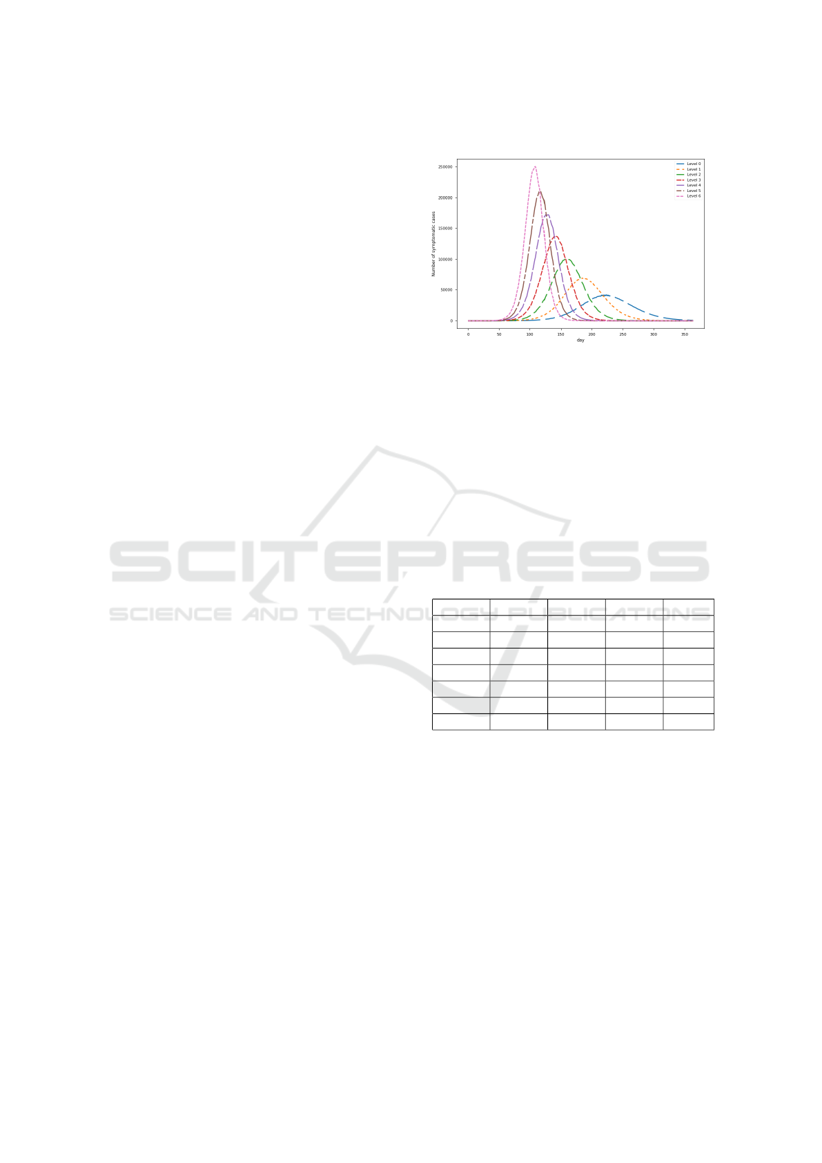
simulations as well as real world epidemics. In Figure

1, We show the average curve of the newly infected

symptomatic cases recorded every day for each level.

As the graph shown, the higher the level, the higher

as well as the earlier the peak is.

Figure 1: Epidemic curves.

In Table 1, we show the statistical characteristics

of the peak epidemics in each level. We can see that

the standard deviation of the peak value for each level

does not differ too much. However, the mean value

of the peak value varies signiﬁcantly. In this table, Pr

99 and Pr 1 represent the value of the 99-percentile

and 1-percentile, respectively. The 1-percentile peak

value of level 0 and level 1 is 10 and 13 respectively.

We note that 10 index cases are created at the begin-

ning of the simulation and the peak value close to 10

actually means virus dose not spread far and the epi-

demic stops early.

Table 1: Level information.

Pr 99 Pr 1 Mean Std

Level 0 61239 10 50035 10921

Level 1 96981 13 81858 10968

Level 2 136102 98499 116361 10929

Level 3 177499 134424 158564 9795

Level 4 220326 169046 197707 11529

Level 5 263997 205040 239315 14079

Level 6 292110 237465 272069 11970

Below we provide a detailed account of data pre-

processing for each problem.

Data generation for predict p

trans

. The ﬁrst ex-

periment, we feed the symptomatic cases of the whole

year to the neural network and let it predict the p

trans

level. In this task, the network got 98% accuracy on

the testing data set. Then we moved forward to see

if a good estimation can be achieved as early as pos-

sible. We, thus, only feed the training algorithm the

ﬁrst few weeks, say from 2 weeks to 8 weeks, of sim-

ulation runs, and measure the performance.

Data generation for predict index case. We ran-

domly pick an interval of 49 days within the entire

epidemic and set the number of weeks when the index

case occurred before the interval of 49 days as the tar-

get answer. For example, if we choose the 49-day in-

Study Simulated Epidemics with Deep Learning

233

terval between the fourteenth day to the sixty-second

day of the entire epidemic as the input, the target an-

swer that we want to predict will be two, which means

the index case occurred two weeks before the 49-day

interval, that is, the ﬁrst day of the entire epidemic.

The end of interval is restricted before the peak date

of each epidemic. If the peak date occurs at the ﬁrst 49

days of the entire epidemic, we will simply pick the

ﬁrst 49 days and the target answer will be zero. All of

the experiments of index date prediction use the ﬁxed

data set in order to compare different results.

Data generation for the next day problem.

Instead of directly using the symptomatic cases

recorded every day, we use the difference between

two days as our input in this experiment, that is the

increased or decreased value of each day. If we con-

sider the unit of X-axis is day and Y-axis represents

the original value of symptomatic cases, it is just like

using the slope between two days as our input data to

feed into the network. The target information we want

to predict is also the increased or decreased value

compare to the ﬁnal day of the known information.

In this task, we think the slope of two days may of-

fer more information than the raw value of each day

as the network can learn the increasing or decreasing

slope and get the correct direction of the next one. It

can also deal with the magnitude problem as the range

of the difference value is not that large compare to the

raw value of the symptomatic cases. So we can use

ﬁxed interval here, which is set as 10 people for each

level. In the simulation world, we put the initial in-

fectious cases in the ﬁrst day of the entire epidemic.

But in the real world, it is impossible to know the in-

dex date certainly. In this task, we ﬁrst use the ﬁrst

49-day interval as the input and predict the 50

day

of the epidemic. After getting an acceptable result,

we randomly move forward the starting point of the

49-day interval forward from 0 to 7 days, that is we

uniformly sample an integer from 0 to 7, and use the

sampled number as the starting point of our sequence.

The shifting of the starting point can be interpreted

as a test of the model’s tolerance level about the un-

certainty of the index date. We call such data shifted

data, and the outcome of learning with shifted data is

called the shifted case.

2.3 Deep Learning Architecture and

Experiment Setup

We use Stacked Long Short-Term Memory networks

launched by Keras(Keras, 2015) to set up our predic-

tion network, which is one of the most Recurrent Neu-

ral Networks. Unlike the traditional feed forward neu-

ral network, which can only deal with the current in-

put and output the corresponding results without con-

sidering past information, the design of Long Short-

Term Memory can help us record the previous infor-

mation and use it for the next round. The modules

of Long Short-Term Memory network have a loop to

reuse the previous information and a forget gate to de-

cide whether the information needs to be recorded or

not. It can record the information of last step as well

as the information far before it. Due to the ability of

combining previous information with the current in-

formation, the network is suitable for dealing with the

time series data, hence ﬁts our purpose.

In Figure 2, we show the general network structure

of our experiments. The variable W depends on the

different number of target levels we want to predict

in each experiment. The dropout rate is set as 20%.

We use Adam as optimizer and categorical cross en-

tropy as loss function. The batch size is set as 32 and

the number of epochs is set around 15. The numbers

of parameters are about 362,000 in the ﬁrst LSTM

layer, 160,000 in second LSTM layer, and 2,000 in the

dense layer respectively. The input and output in the

ﬁgure mean the dimension of input and output data of

each layer. All of the inputs fed into the model are the

infected cases.

Figure 2: Network structure.

In the study of epidemics, the severe and urgent

ones need most of the attention. Therefore, in our

study, we sometimes partition training data according

to its severity, that is p

trans

, to build models for each

severity level. We call this leveled training and de-

noted by Level x in the tables in section 3. On the

other hand, when we use training data of all levels to

build one model, the performance of this model facing

SIMULTECH 2019 - 9th International Conference on Simulation and Modeling Methodologies, Technologies and Applications

234

different severity cases is also of interest. The testing

data is thus partitioned according to severity and we

get several testing results. We call this leveled testing

and use Lv x to denote a row is the result of leveled

testing with level x, this notation is only used at the

next day prediction problem.

2.4 Variable Length Interval

As the range of the peak value is too large, from ten

to about thirty thousand. If we directly transfer them

into categories and apply one hot encoding on them.

The target answer will be too sparse and the accuracy

will be really low. We also tried to predict the peak

value directly without any classiﬁcation but it ended

up with the result of very large mean squared error

and the network learned nothing. For this task, if we

use ﬁxed interval to convert the value, one hundred by

each level for example, it does not make sense as the

error of one hundred is different for the basic number

with two hundred and twenty thousand. So we con-

duct a method to convert the value of symptomatic

cases into several levels. We separate each level ac-

cording to the magnitude of the value. We want each

level to have a ﬁxed percentile of the median value

in a level, not a ﬁxed range of value for every levels.

The following is the formula of the conversion. The

range of the interval will become larger as the value

raises. And the median of each level is a geometric

series with the ratio of (1+α) / (1-α), the variable α is

the percentage of error we can accept. We set a basic

number β as the median of the ﬁrst interval. And the

value below the basic number will be viewed as the

level 0. At this experiment, we set the basic number

β as one hundred and acceptable percentage α as 5%

and 10%.

Level = blog

(1+α)

(1−α)

PeakValue

+ 1.5c (1)

2.5 Measurements

To evaluate the utility of trained models, we have to

incorporate the requirements of real applications into

the measurements. For example, to predict the peak

date, it is acceptable to be off one or two days since

the peak date might be for the logistic planning or

speculating the potential impact on the healthcare de-

livery system. Therefore, a close enough prediction

is acceptable. Let L = {`

,...,`

k−1

} be the k set of

possible predictions. Let U = L × L → [0, 1] be the

utility function, and U(`

) = 0.8 means that the

utility for the case that the model predicted `

while

the true case is `

is 0.8. Given a case with true label

and the prediction is (p

,..., p

k−1

), the utility is

∑

k−1

j=0

L( j,i)p( j). And the utility of a dataset is the av-

erage utility of each case in that dataset. The utility of

the model for a dataset is the expected utility, In this

paper, we use numerical values as symbols for `s, and

take the advantage that we can treat them as numer-

ical values so that arithmetic operations are possible.

Usually, the utility depends on the distance between

the predicted value and true value. For example, if the

predicted peak day is off by one day the utility is very

high or as good as the correct predictions. For those

situations, we can simplify the utility function to an

utility array U = (u

−k+1

,...,u

k−1

) where the

subscript is the value of predicted index minus true

index. Therefore, u

is always 1. We use Acc ± 1

(Acc ±3) to denote the case that the immediate neigh-

bors(two neighbors) are considered correct prediction

respectively.

Given a value α, ∆

is the minimum d such that

the utility array with width 2d + 1 has utility no less

than α and use ∆

= ±d. In this paper, we use ∆0.9

and ∆0.95 to denote ∆

0.9

and ∆

0.95

when they appear

in the head row of a table.

When ﬁxed length intervals are used for categoriz-

ing numerical data and when the range of the values

is large. The error in the absolute sense may not tell

the whole story. For each testing case, we deﬁne the

relative error as follows: re(`,tv) = |v(`) − tv|/v(`),

where ` is the predicted level, tv is the true value

and v() is a mapping from level to a numerical level,

here we choose the middle point of the interval. We

can then compute the mean relative error as the mean

value of the relative errors of all cases.

3 RESULTS

For each experiment, we ﬁrst use the training data

of all levels to build the model for prediction. And

the result is identiﬁed as over all in the table below.

We then study the cases that given the ﬁxed p

trans

level, how well the algorithms can learn. That is we

train seven different models individually, one for each

level. And we identify the results with the order of

level , that is the row level i in the table contains the

performance on each level. And all of the results re-

ported below comes from testing data, which has not

been seen by the model.

3.1 p

trans

In the experiments of p

trans

prediction, the dataset

contains ﬁfty thousand records with p

trans

range from

0.075 to 0.105, divided into 7 levels.

Study Simulated Epidemics with Deep Learning

235

The retrospective estimation of p

trans

performs

well, the accuracy is higher than 98%, and the pre-

diction is off by at most one level. For the perspective

case, we carry out the experiment which uses ﬁrst two

weeks data, that is to predict p

trans

after 2 weeks of

the epidemic, up to ﬁrst eight weeks. As the results

shown in Table 2, two weeks data is enough to reach

over 60% accuracy and almost 80% of the cases is off

by one level and for the 8 week experiment, we have

over 97% accuracy within an error of one level. It is

worth noting that from 2 weeks to 8 weeks the growth

of the accuracy is almost a line as shown in Figure 3.

Table 2: Ptrans prediction.

Accuracy Acc±1 ∆0.9 ∆0.95

52 wks 98.471% 99.928% ±0 ±0

2 wks 60.685% 78.844% ±3 ±3

3 wks 61.908% 82.869% ±2 ±3

4 wks 65.627% 88.953% ±2 ±2

5 wks 69.907% 92.724% ±1 ±2

6 wks 72.995% 95.689% ±1 ±1

7 wks 75.940% 96.938% ±1 ±1

8 wks 78.742% 97.238% ±1 ±1

Figure 3: p

trans

prediction accuracy.

3.2 Peak Date

The unit for peak date prediction is day, that is each

level corresponds to one day. Although the overall

accuracy is only 50%, and ∆0.9 = ±17 as shown in

Table 3. However, we note that the prediction is done

at the end of the 7

week, which is quite early.

The results of level here is leveled learning as we

mentioned above. And the following level results are

the same as this experiment except for the next day

prediction experiment. We separate the data of each

level ﬁrst then split the training and testing data to

train a model for each level. When we train different

models for different level of p

trans

, we note that in Ta-

ble 3 for higher level (level 3 to level 6) the prediction

is off by at most a week 95% of times.

Table 3: Peak date prediction.

Accuracy Acc±3 ∆0.9 ∆0.95

Level 0 57.919% 58.781% ±21 ±24

Level 1 60.636% 63.221% ±11 ±14

Level 2 63.949% 69.781% ±7 ±10

Level 3 63.287% 72.829% ±7 ±7

Level 4 63.660% 75.464% ±7 ±7

Level 5 68.522% 83.168% ±4 ±7

Level 6 62.698% 78.042% ±4 ±6

Overall 56.507% 63.232% ±17 ±28

3.3 Peak Value

The peak value is deﬁned as the largest number of

people infected in one day for the entire epidemic pe-

riod. As mentioned above that we use variable length

interval to partition peak values. The beneﬁt of it is

that this formulation corresponding to the relative er-

ror which suits our purpose better. However, one of

the drawback is the interpretation of the results need a

little more works. We carry out two experiments with

different variable length intervals, α = 0.1 (shown in

Table 4) and α = 0.05 (shown in Table 5) respectively.

It is expected that the accuracy for α = 0.05 case is

lower than α = 0.1 case, because it has smaller rela-

tive error. To be correct for the 0.05 case, the predic-

tion can not be off over 5%, while for 0.1 case it can

be off by as large as 10%. Roughly, for the 0.05 case,

Acc ± 1 = 0.96, means that 96% of predictions is off

by at most 15%. We can see that setting α to 0.05

produce better results at higher level.

Table 4: Peak value prediction α = 0.1.

Accuracy Acc±1 ∆0.9 ∆0.95

Level 0 70.377% 93.837% ±1 ±2

Level 1 76.011% 99.801% ±1 ±1

Level 2 79.722% 100% ±1 ±1

Level 3 76.739% 99.933% ±1 ±1

Level 4 84.350% 100% ±1 ±1

Level 5 84.625% 99.933% ±1 ±1

Level 6 81.084% 100% ±1 ±1

Overall 68.062% 88.994% ±2 ±2

Table 5: Peak value prediction α = 0.05.

Accuracy Acc±1 ∆0.9 ∆0.95

Level 0 61.962% 79.059% ±2 ±3

Level 1 63.029% 85.355% ±2 ±2

Level 2 62.624% 90.656% ±1 ±2

Level 3 66.402% 96.090% ±1 ±1

Level 4 70.225% 96.021% ±1 ±1

Level 5 71.239% 95.692% ±1 ±1

Level 6 75.661% 99.603% ±1 ±1

Overall 58.514% 75.461% ±3 ±5

SIMULTECH 2019 - 9th International Conference on Simulation and Modeling Methodologies, Technologies and Applications

236

3.4 Infected Cases of Next Day

We try to study the possibility to build an online sys-

tem to predict the number of newly infected cases

based on the current situation. We ﬁrst study the sim-

plest version of the problem, i.e., predict the outcome

of the 50

day given ﬁrst 49 days. We call it ﬁxed

case, since the ﬁrst data item corresponding to a ﬁxed

day, in this case ﬁrst day, of the simulation. One way

to interpret the ﬁxed case is that we know the index

date exactly. Next, we study the scenario that we are

not sure about the index date, but we know that index

date is in a time interval. In our experiment, for each

simulation run, we generate 7 sequences of length 49,

where the starting day ranged from the 1

day to the

day. This version is called shift window case.

Training starts with a preprocessing process, we

take the difference of the values of two consecutive

days to form a new sequence as the input to the learn-

ing algorithm, and the label is the difference between

next day and the last day in the input. The model

learns together with a postprocessing, that is adding

the value predicted with the value of last day in the

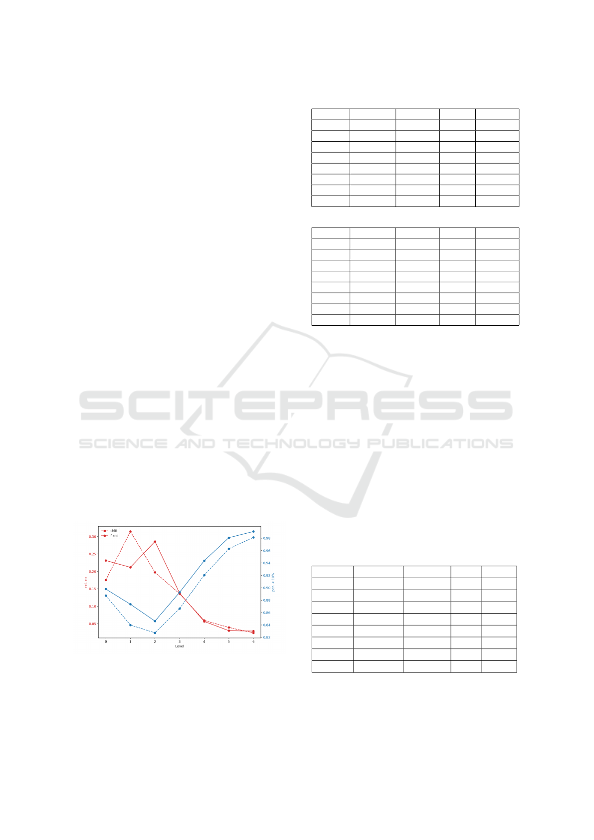
input. As shown in Figure 4, the accuracy and Acc±3

decrease as the testing level increase, the reason is that

we categorized the value with ﬁxed length intervals.

When the level increases, a more infectious virus, the

newly infected cases also increase, thus more difﬁcult

to predict the category correctly. Overall, the ﬁxed

model performs better, except slightly higher mean

relative error as shown in Figure 4. This conﬁrms our

intuition that the shift window version is harder than

the ﬁxed one. Overall, the mean relative error is less

than 15% and almost 90% of the cases the prediction

is at most 10 % off the mark. We note that for more

severe epidemic, higher level ones, the mean relative

error is less than 6% as shown in Table 6 and 7.

Figure 4: Rel. err and per. below 10% of shift and ﬁxed

data.

Table 6: Next day prediction (shift window).

Accuracy Acc±3 rel. err ≤10%

Lv 0 87.064% 96.054% 0.175 88.730%

Lv 1 76.521% 93.640% 0.314 83.987%

Lv 2 64.218% 89.874% 0.197 82.729%

Lv 3 56.685% 84.461% 0.136 86.647%

Lv 4 50.411% 75.920% 0.059 92.036%

Lv 5 48.045% 68.590% 0.039 96.290%

Lv 6 47.525% 61.999% 0.024 98.129%

Overall 62.570 % 83.005% 0.143 89.153%

Table 7: Next day prediction (ﬁxed).

Accuracy Acc±3 rel. err ≤10%

Lv0 88.667% 96.288% 0.231 89.794%

Lv1 81.908% 94.102% 0.211 87.342%

Lv2 68.986% 92.710% 0.285 84.625%

Lv3 60.569% 89.993% 0.137 89.264%

Lv4 55.238% 83.289% 0.056 94.363%

Lv5 52.087% 76.076% 0.030 98.078%

Lv6 51.455% 70.105% 0.029 99.074%

Overall 66.642% 87.307% 0.148 91.232%

3.5 Index Date

Last, we study the problem that given a segment of

an epidemic, predicting how far is the ﬁrst day in the

sequence from the ﬁrst date of the epidemic. And we

set the unit of prediction to be week. As show in Ta-

ble 8, the over all accuracy is not impressive although

we already set the predicting unit to week, instead

of day in the case for predicting peak date. We do

note a recurrent scenario also show in Table 8, that

the model trained with higher level of p

trans

performs

better than lower level cases. Although, it is too early

to claim that this is a difﬁcult task to build a prediction

model. We do want to mention that a negative result

with simulated data, can be seen as a indication to the

difﬁculty of the problem in real world. Because the

real world data is much more chaotic with inﬁnitely

many sources of noises.

Table 8: Index date prediction.

Accuracy Acc±1 ∆0.9 ∆0.95

Level 0 24.254% 49.901% ±5 ±7

Level 1 26.508% 64.016% ±3 ±4

Level 2 38.436% 78.794% ±2 ±3

Level 3 52.154% 88.867% ±2 ±2

Level 4 60.146% 90.981% ±1 ±2

Level 5 66.534% 96.156% ±1 ±1

Level 6 70.504% 96.825% ±1 ±1

Overall 39.397% 69.509% ±4 ±7

Study Simulated Epidemics with Deep Learning

237

4 CONCLUSION AND FUTURE

WORKS

The preliminary results are promising. It is worth

pointing out that when the infectiousness is low, i.e.,

the p

trans

at lower level, the disease control agency

only has to monitor its progress, when the infectious

is very high, there is not much the agency can do.

Therefore, the interesting cases are those in the mid-

dle. We note that the prediction is more accurate with

higher level infectiousness. Also our choice of the

utility functions more or less reﬂect the real applica-

tions. For the prediction of peak value, we do not

use ﬁx length partition, which corresponding to the

idea of absolute error. Instead, we use variable length

interval, which is corresponding to relative error. We

believe this trick can be applied elsewhere. When pre-

dicting next day, we feed the model with the sequence

of the differences between two consecutive days, this

corresponding to take the derivative of the epidemic

curve at given day. This is also an interesting trick

which might be useful in other situations. We note

that the deep learning performed not so well for pre-

dicting the index date. One possible interpretation is

that this is really a difﬁcult problem even in the sim-

pliﬁed simulated world. The hope to get a good esti-

mation in the real world might even be more difﬁcult.

Therefore, a not so positive result can shed light on the

limitation of what can be learnt in real world and we

might want to frame the problem differently to hope

for better results.

We plan to try other machine learning approaches,

especially regression based ones like SVR so that one

might get better understanding about the capacity and

limitation of deep learning methods on simulated epi-

demiology data. From disease control perspective,

one obvious future direction is to include mitigation

strategies, such as vaccination, and social distancing

so that the outcome of various combination of miti-

gation can be learned. The parameter spaces will be

much larger when mitigation strategies included, and

the power of deep learning can be further explored.

To use more detailed information of a simulated epi-

demic, such as geographic location is also an inter-

esting and important next step. Furthermore, how to

apply the trained model in the real situation, is also a

very important yet challenging problem. We can start

by introducing additive random noise to the output of

simulation system to mimic the background or base-

line disease states in real world and feed the perturbed

data into the learning system. One exciting idea is

to use the generative adversarial model (Goodfellow

et al., ) to train a generative model to generate simu-

lation results without running the simulation.

ACKNOWLEDGEMENTS

This study is supported in part by MOST, Tai-

wan, Grant No. MOST107-2221-E-001-017-MY2

and MOST107-2221-E-001-005 and by Multidisci-

plinary Health Cloud Research Program: Technology

Development and Application of Big Health Data,

Academia Sinica, Taipei, Taiwan.

REFERENCES

Anderson, R. and May, R. (1992). Infectious Diseases of

Humans: Dynamics and Control. Dynamics and Con-

trol. OUP Oxford.

Chang, H.-J., Chuang, J.-H., Fu, Y.-C., Hsu, T.-S., Hsueh,

C.-W., Tsai, S.-C., and Wang, D.-W. (2015). The im-

pact of household structures on pandemic inﬂuenza

vaccination priority. In SIMULTECH2015, pages

482–487.

Fu, Y.-c., Wang, D.-W., and Chuang, J.-H. (2012). Rep-

resentative contact diaries for modeling the spread of

infectious diseases in taiwan. PLoS ONE, 7(10):1–7.

Germann, T. C., Kadau, K., Longini, I. M., and Macken,

C. A. (2006). Mitigation strategies for pandemic in-

ﬂuenza in the United States. Proceedings of the Na-

tional Academy of Sciences, 103(15):5935–5940.

Goodfellow, I., Pouget-Abadie, J., Mirza, M., Xu, B.,

Warde-Farley, D., Ozair, S., Courville, A., and Ben-

gio, Y. Generative adversarial nets. In Advances in

Neural Information Processing Systems 27.

Keras (2015). Keras documentation. https://keras.io/.

Li, M. and Vitnyi, P. M. (2008). An Introduction to Kol-

mogorov Complexity and Its Applications. Springer.

Mnih, V., Kavukcuoglu, K., Silver, D., Graves, A.,

Antonoglou, I., Wierstra, D., and Riedmiller, M. A.

(2013). Playing atari with deep reinforcement learn-

ing. CoRR, abs/1312.5602.

Tsai, M.-T., Chern, T.-C., Chuang, J.-H., Hsueh, C.-W.,

Kuo, H.-S., Liau, C.-J., Riley, S., Shen, B.-J., Shen,

C.-H., Wang, D.-W., and Hsu, T.-S. (2010). Efﬁcient

simulation of the spatial transmission dynamics of in-

ﬂuenza. PLOS ONE, 5(11):1–8.

SIMULTECH 2019 - 9th International Conference on Simulation and Modeling Methodologies, Technologies and Applications

238