
Design of a Self-tuning Predictive PI Controller for Delay Systems based
on the Augmented Output
Yoichiro Ashida
1 a
, Shin Wakitani
2 b
and Toru Yamamoto
2 c
1
Department of Electrical Engineering and Computer Science, National Institute of Technology,
Matsue College, 14-4 Nishiikumacho, Matsue, Japan
2
Graduate School of Engineering, Hiroshima University, 1-4-1 Kagamiyama, Higashi-hiroshima, Japan
Keywords:
Predictive PI Controller, Predictive Control, Delay System, Data-driven, Self-tuning.
Abstract:
This paper proposes an online type control parameter tuning method for a predictive PI controller. Predictive
PI controller is based on a PI controller with a Smith predictor, and it is effective for a controlled object with
large dead-time. Control performance of the predictive PI controller strongly depends on control parameters.
Recently, some data-driven controller tuning methods have been proposed. The methods directly calculate
suitable parameters from one or some sets of operating data. In addition, almost controlled processes are
time-variant. In this paper, a data-driven self-tuning predictive PI controller is proposed. The effectiveness of
the proposed scheme is evaluated by a simulation example.
1 INTRODUCTION
PID controllers(Astrom and Hagglund, 2005; Berner
et al., 2018) are often applied in industries. Espe-
cially in chemical process systems, 90% or more of
controllers are PID controllers. However, according
to some surveys, most of the employed PID form
controllers are PI controllers(Bialkowski, 1993; Sun
et al., 2016). One of the reasons is the difficulty of
tuning of derivative gains. To obtain good control
performance for a controlled object with a long dead-
time, the derivative gain should be large. However,
the larger the derivative gain is, the stronger the influ-
ence of noise is. This is because a derivative element
amplifies high-frequency signals. Therefore, it is dif-
ficult to tune derivative gain suitably than the other
gains.
Lots of controllers which can obtain good con-
trol performance for a dead-time system are pro-
posed. Representative examples are Smith pre-
dictors(Ingimundarson and Hagglund, 2001; Sanz
et al., 2018) and model predictive controllers
(MPC)(Rawlings and Mayne, 2009; Gallego et al.,
2019). The Smith predictor constructs positive feed-
back for a conventional controller like a PI controller.
a
https://orcid.org/0000-0001-7751-5270
b
https://orcid.org/0000-0002-3850-3864
c
https://orcid.org/0000-0001-6500-8394
By the Smith predictor, dead-time of a controlled sys-
tem is removed from a closed-loop. Therefore, the
conventional controller can be designed for a system
without a dead-time. A MPC needs a mathematical
model of the process. The input value is calculated
based on an output of the mathematical model. These
MPCs are sometimes employed in industries. How-
ever, both controllers predict future output, and accu-
racy of a mathematical model strongly affects con-
trol performance. Separately, a predictive PI con-
troller(Hagglund, 1992; Airikka, 2014; Hassan et al.,
2016) has been proposed. Although the predictive PI
controller is a combination of a PI controller and a
Smith predictor, a mathematical model is not required
overtly and has only four parameters. Authors also
propose a tuning scheme of the predictive PI con-
troller(Ashida et al., 2019), and effectiveness for a
noisy system is shown by comparing a PID controller.
Recently, data-driven controller tuning methods
are proposed. According to the conventional con-
troller parameters tuning methods, the parameters are
determined based on a mathematical model of a con-
trolled system. In contrast, data-driven methods di-
rectly compute the control parameters without any
system model. Therefore, the methods can reduce
the cost of the modeling and attract attention. Rep-
resentative examples are Iterative Feedback Tuning
(IFT)(Hjalmarsson et al., 1998; Wang and Ma, 2015),
Virtual Reference Feedback Tuning (VRFT)(Campi
672
Ashida, Y., Wakitani, S. and Yamamoto, T.
Design of a Self-tuning Predictive PI Controller for Delay Systems based on the Augmented Output.
DOI: 10.5220/0007919306720679
In Proceedings of the 16th International Conference on Informatics in Control, Automation and Robotics (ICINCO 2019), pages 672-679
ISBN: 978-989-758-380-3
Copyright
c
2019 by SCITEPRESS – Science and Technology Publications, Lda. All rights reserved

et al., 2002; Campestrini et al., 2016) and Fictitious
Reference Iterative Tuning (FRIT)(Soma et al., 2004;
Kaneko, 2015). Among the data-driven methods,
FRIT method requires only one set of input/output
data, and some examples of actual systems are re-
ported. However, these methods determine one set
of controller parameters, and it is difficult to main-
tain control performance for a time-variant system.
To tackle this problem, data-driven tuning methods
are extended to some self-tuning controllers. Au-
thors also propose a data-driven PID controller tuning
method(Ashida et al., 2016), and the method is ex-
tended to the self-tuning PID controller(Ashida et al.,
2017).
In this paper, a self-tuning predictive PI controller
is proposed. The proposed controller is an extent
of a self-tuning PID controller proposed by the au-
thors(Ashida et al., 2017). A recursive least squares
method(Goodwin and Sin, 1984) is employed as an
adaptive algorithm. In the second section, a predic-
tive PI controller is derived from a PI controller with
a Smith predictor. In addition, it is proved that the
predictive PI controller can realize complete model
matching for a first-order system with a dead-time.
In the third section, the proposed design method of a
self-tuning predictive PI controller is described. Data-
driven controller parameters tuning method is firstly
explained. Next, an extension of the self-tuning con-
troller is described. At last, the proposed control
scheme is evaluated by some simulation and experi-
mental results.
2 DISCRETE-TIME PREDICTIVE
PI CONTROLLER
In this section, a discrete-time predictive PI control
law is derived. The predictive PI controller is based
on a PI controller with a Smith predictor. At first, a
controlled object G(z
−1
) is assumed to be the follow-
ing first-order system:
G(z
−1
) = G
p
(z
−1
)z
−d
, (1)
where G
p
(z
−1
) denotes a delay element of the sys-
tem, and d denotes a dead-time which is known. A
PI controller with Smith predictor can be expressed
as follows:
u(t) =
K
P
+
K
I
∆
n
e(t) − G
p
(z
−1
)
z
−d
− 1
u(t)
o
,
(2)
where K
P
, K
I
and u(t) denote a proportional gain, an
integral gain and an input signal. ∆ denotes the differ-
encing operator defined by ∆ := 1 −z
−1
, where z
−1
is
the shift operator which means z
−1
y(k) = y(k −1). In
addition, u(t) also denotes a controlled input, and e(t)
denotes a controlled error defined as follows:
e(t) := r(t) − y(t), (3)
where r(t) and y(t) denote a reference signal and an
output signal respectively. G
p
(z
−1
) is assumed to be
the following first-order system:
G
p
(z
−1
) =
z
−1
b
0
1 + a
1
z
−1
. (4)
By substituting (4), (2) can be rewritten as follows:
u(t) =
K
P
+
K
I
∆
e(t)
+
z
−1
b
0
(K
P
∆ + K
I
)
∆(1 + a
1
z
−1
)
(z
−d
− 1)u(t). (5)
Next, PI gains K
P
and K
I
are set as follows:
K
P
= −
a
1
b
0
K
pred
K
I
=
1
b
0
K
pred
, (6)
where K
pred
is a prediction gain. By substituting (6)
to (5), the following predictive PI control law is ob-
tained:
u(t) =
K
P
+
K
I
∆
e(t) +
z
−1
K
pred
∆
(z
−d
− 1)u(t).
(7)
To control a first-order system with delay shown
in (1) and (4) by the predictive PI controller, a closed-
loop transfer function is as follows:
W (z
−1
) =
K
pred
(1 + a
1
z
−1
)z
−(d+1)
1 + (K
pred
− 1 +a
1
)z
−1
+ a
1
(K
pred
− 1)z
−2
. (8)
The transfer function is simplified using (6). A pre-
diction gain K
pred
is set as follows:
K
pred
= 1 + p
1
, (9)
where p
1
is a value included in a following first-order
reference model with a dead-time:
G
m
(z
−1
) :=
1 + p
1
1 + p
1
z
−1
z
−(d+1)
. (10)
p
1
is an user-specified parameter and determines a
rise-time. By substituting (9) to (8), the closed-loop
transfer function is rewritten as follows:
W (z
−1
) =
(1 + p
1
)(1 + a
1
z
−1
)
1 + (p
1
+ a
1
)z
−1
+ p
1
a
1
z
−2
z
−(d+1)
=
1 + p
1
1 + p
1
z
−1
z
−(d+1)
. (11)
Design of a Self-tuning Predictive PI Controller for Delay Systems based on the Augmented Output
673

Therefore, the predictive PI controller can control a
first-order system with a dead-time as a first-order
reference model. When a controlled object has high-
order characteristics strongly, control performance of
the predictive PI controller deteriorates. Therefore,
the controller should be applied for a system like a
first-order system.
3 DESIGN OF A DATA-DRIVEN
SELF-TUNING PREDICTIVE PI
CONTROLLER
According to (6) and (9), a predictive PI controller
can be designed if system parameters are known. To
obtain the system parameters, system modeling is
required. However, it takes considerable burden to
make a mathematical model. In this paper, a data-
driven controller design method is employed to deter-
mine controller parameters. The method calculates
the controller parameters directly from a set of in-
put/output data. In addition, the controller parameter
tuning method is extended to a self-tuning controller
by employing a recursive least squares method.
The predictive PI control law shown in (7) can be
rewritten as follows:
r(t) =
1
K
P
∆ + K
I
∆u(t) + y(t)
+
K
pred
K
P
∆ + K
I
{u(t − 1) − u(t −d − 1)}. (12)
Augmented output φ(t) is defined as
φ(t) =
1
K
P
∆ + K
I
∆u(t) + y(t)
+
K
pred
K
P
∆ + K
I
{u(t − 1) − u(t −d − 1)}. (13)
From the definition, the following relationship is ob-
tained;
φ(t) = r(t). (14)
In the proposed method, it is desired to make the
system output y(t) tracks the reference model output
y
m
(t) which is defined as
y
m
(t) = G
m
(z
−1
)r(t), (15)
where G
m
(z
−1
) has been already defined by (10), and
p
1
is determined using the following formulation:
p
1
= −exp
−
T
s
T
m
. (16)
T
m
denotes a time-constant of the reference model
G
m
(z
−1
). The evaluation function J is defined as fol-
lows:
J =
N
∑
j=0
ε( j)
2
, (17)
where N denotes the number of data and ε(t) is de-
fined as follows:
ε(t) = y(t) −G
m
(z
−1
)φ(t), (18)
where optimized parameters are K
P
and K
I
. It is not
required to search K
pred
because K
pred
depends only
on p
1
of reference model G
m
(z
−1
). By minimizing
the evaluation function J, G
m
(z
−1
)φ(t) becomes iden-
tical to y(t). When the minimization has been finished
enough, the following relationship can be obtained:
G
m
(z
−1
)φ(t) = y(t). (19)
By using a relationship as (14), the following relation
can be obtained:
y(t) = G
m
(z
−1
)r(t). (20)
Therefore, the controlled output becomes identical to
the reference model output using optimized controller
parameters.
The above discussions are based on deterministic
systems. However, actual systems are stochastic sys-
tems. To reduce the influence of noise, the filtered
input/output signals u
f
(t) and y
f
(t) are used. A de-
lay part of the reference model is used as a filter, thus
u
f
(t) and y
f
(t) are defined as follows.
y
f
(t) :=G
mp
(z
−1
)y(t), (21)
u
f
(t) :=G
mp
(z
−1
)u(t). (22)
G
mp
(z
−1
) denotes a delay part of the reference model
as follows:
G
m
p(z
−1
) =
1 + p
1
1 + p
1
z
−1
z
−1
. (23)
From a view of the frequency domain, φ(t) is band-
limited by the reference model and ε(t) is composed
with band-limited φ(t) in the proposed tuning scheme.
Therefore, the reference model filter not only reduces
the influence of noise but also emphasizes the impor-
tant band of the signal. Hereinafter u
f
(t) and y
f
(t)
are used instead of u(t) and y(t).
In this paper, a self-tuning predictive PI controller
is designed by employing recursive least squares
(RLS) method(Goodwin and Sin, 1984). However,
the evaluation function J cannot be minimized by
RLS method because ε(t) is not linear to optimized
ICINCO 2019 - 16th International Conference on Informatics in Control, Automation and Robotics
674

parameters K
P
and K
I
. By multiplying K
P
∆ + K
I
to
(18), the following relation is obtained:
(K
P
∆ + K
I
)ε(t) =(K
P
∆ + K
I
)y
f
(t)
+ G
m
(z
−1
)(K
P
∆ + K
I
)φ(t). (24)
Based on (24),
˜
ε(t) is defined as
˜
ε(t) = (K
P
∆ +
K
I
)ε(t), and it can be rewritten as follows:
˜
ε(t) =G
m
(z
−1
)[∆u
f
(t)
+ K
pred
{u
f
(t − 1) − u
f
(t − d − 1)}]
− a
1
{y
f
(t) − G
m
(z
−1
)y
f
(t)}
− a
2
{G
m
(z
−1
)y
f
(t − 1) − y
f
(t − 1)}, (25)
where a
1
and a
2
are optimized parameters and defined
as follows:
a
1
:= K
P
+ K
I
a
2
:= K
P
. (26)
As a result, a new evaluation function is defined as
follows:
˜
J =
1
N
N
∑
j=0
˜
ε( j)
2
. (27)
˜
ε(t) is linear to a
1
and a
2
, then a minimization of
˜
J
is a least squares problem. a
1
and a
2
are calculated
recursively using the following recursive least squares
algorithm, and a
1
and a
2
are converted to K
P
and K
I
by (26).
ˆ
θ(t) =
ˆ
θ(t − 1) + K(t)
˜
ε(t), (28)
K(t) =
P(t − 1)ϕ(t)
ω + ϕ
T
(t)P(t − 1)ϕ(t)
, (29)
P(t) =
1
ω
P(t − 1) −
P(t − 1)ϕ(t)ϕ
T
(t)P(t − 1)
ω + ϕ
T
(t)P(t − 1)ϕ(t)
,
(30)
where ω is a forgetting factor, and
˜
ε(t), θ(t) and ϕ(t)
are calculated as follows:
˜
ε(t) :=G
m
(z
−1
)[∆u
f
(t)
+ K
pred
{u
f
(t − 1) − u
f
(t − d − 1)}]
−
ˆ
θ
T
(t − 1)ϕ(t) (31)
ˆ
θ(t) :=[ ˆa
1
(t), ˆa
2
(t)]
T
, (32)
ϕ(t) :=[y
f
(t) − G
m
(z
−1
)y
f
(t),
G
m
(z
−1
)y
f
(t − 1) − y
f
(t − 1)]
T
. (33)
An initial value of covariance matrix P(t) and
ˆ
θ(t)
which is estimated vector of a
i
(t) are determined by
the following equations:
P(0) =αI (34)
ˆ
θ(0) =[ ˆa
1
(0), ˆa
2
(0)]
T
, (35)
Figure 1: Block diagram of the proposed self-tuning con-
troller.
where α is determined under a condition of α > 0, and
I is a 2 × 2 matrix.
A block diagram of the proposed scheme is shown
in Fig. 1. A predictive PI controller can be divided
into a PI controller and a predictor. K
P
and K
I
are the
optimized parameters, thus only PI controller is tuned
recursively and the predictor is fixed.
4 SIMULATION RESULT
In this section, the proposed controller is evaluated by
the following time-variant system.
(i) t ≤ 3500
G(s) =
390s + 260
35s
4
+ 209s
3
+ 418s
2
+ 316s +7
e
−100s
,
(36)
(ii) t > 3500
G(s) =
312s + 208
70s
4
+ 418s
3
+ 836s
2
+ 632s +14
e
−100s
.
(37)
The system is discretized by T
s
= 1 s and the follow-
ing discrete system can be obtained:
(i) t ≤ 3500
y(t) =1.33y(t − 1) −0.41y(t − 2) + 0.07y(t −3)
− 0.003y(t − 4) +0.55u(t − 101)
+ 0.36u(t − 102) −0.29u(t − 103)
− 0.02u(t − 104) +ξ(t), (38)
(ii) t > 3500
y(t) =1.33y(t − 1) −0.41y(t − 2) + 0.07y(t −3)
− 0.003y(t − 4) +0.28u(t − 101)
+ 0.18u(t − 102) −0.15u(t − 103)
− 0.01u(t − 104) +ξ(t), (39)
where ξ(t) denotes the Gaussian white noise sequence
with zero mean and variance 0.1
2
. A reference model
Design of a Self-tuning Predictive PI Controller for Delay Systems based on the Augmented Output
675
0 1000 2000 3000 4000 5000 6000 7000 8000 9000 10000
-50
0
50
100
150
y
Reference signal
Output
Reference trajectory
0 1000 2000 3000 4000 5000 6000 7000 8000 9000 10000
Time [step]
-5
0
5
10
15
u
Figure 2: Control result using the proposed method.
0 1000 2000 3000 4000 5000 6000 7000 8000 9000 10000
-0.05
0
0.05
0.1
0.15
K
P
0 1000 2000 3000 4000 5000 6000 7000 8000 9000 10000
Time [step]
-2
0
2
4
6
K
I
10
-3
Figure 3: Trajectories of the control parameters correspond-
ing to Fig. 2.
was determined as the following system:
G
m
(z
−1
) =
0.05z
−1
1 − 0.95z
−1
z
−100
, (40)
where time-constant was set as T
m
= 20 s and dead-
time was set as known. The control result using the
proposed method is shown in Fig. 2, and trajectories
of the controller parameters are also shown in Fig. 3.
Parameters of RLS method was as follows:
α = 1, ω = 0.995. (41)
Before and after the characteristics of the system
were changed, a good control performance was ob-
tained. From Fig. 3, the PI gains were tuned adap-
tively after the varying of the controlled object. How-
ever, just after the varying of the system, the PI pa-
rameters did not converge quickly, and the control
performance was strongly deteriorated. It is future
work to solve the problem.
At last, influence of the time-constant of the refer-
ence model is discussed. Figure 4 shows the control
0 1000 2000 3000 4000 5000 6000 7000 8000 9000 10000
0
20
40
60
80
100
120
y
T
m
= 0.1 T
m
= 20 T
m
= 100
0 1000 2000 3000 4000 5000 6000 7000 8000 9000 10000
Time [step]
0
5
10
15
20
25
u
T
m
= 0.1 T
m
= 20 T
m
= 100
Figure 4: Controlled outputs corresponding to the time-
constant of the reference model.
outputs when T
m
were set as 0.1, 20, and 100. The
reference signal and designed parameters except the
reference model were the same as Figure 2. When
T
m
= 20, the result is likely the same as 2, and when
T
m
= 100, there were no overshoots. However, the
output sometimes became spike-like when T
m
= 0.1.
In this simulation, there is a mismatch. The reason
of the mismatch is that the controlled object is high-
order although the predictive PI controller is designed
for a first-order system. From Figure 4, the influence
of the mismatch tends to be larger as T
m
becomes
smaller. Therefore, it is recommended that a refer-
ence model with the slow response should be applied
firstly, and T
m
should become smaller gradually in an
actual usage.
5 EXPERIMENTAL RESULT
In this section, a pilot-scale tank system is used to
evaluate the proposed method under the condition
more realistic than the simulation example. Fig. 5
shows an appearance of the system, and the corre-
sponding schematic figure is illustrated in Fig. 6. The
controlled object is to regulate the temperature of the
mixed water. There are two valves which regulate the
flow of the cold and hot water respectively. In this re-
sult, the opening ratio of the cold water’s valve u
c
(t)
was constant as 40%. A predictive PI controller deter-
mined the opening ratio of the hot water’s valve u
h
(t)
to regulate the temperature. In this section, a sam-
pling time T
s
is 5 s. The experimental system has a
transfer delay as a dead-time. The delay is about 30
seconds. In addition, a time-constant is about 30 sec-
onds. Therefore, ratio of dead-time and time-constant
is about 1. A control result by using the proposed
method is shown in Fig. 7, and the trajectories of the
ICINCO 2019 - 16th International Conference on Informatics in Control, Automation and Robotics
676

Cold water Hot water
Tank
Thermometer
Figure 5: Appearance of the experimental temperature con-
trol system.
M
D/A
Computer
A/D
M
Cold Water
Hot water
Resistance thermometer
Tank
Figure 6: Schematic figure of the experimental temperature
control system.
PI gains are also shown in Fig. 8. In this result, pa-
rameters of the proposed method were set as follows:
α = 100, ω = 0.995. A reference model was deter-
mined as the following system:
G
m
(z
−1
) =
0.22z
−1
1 − 0.78z
−1
z
−7
, (42)
where time-constant was set as 20 s and dead-time
was set as d = 7. It is difficult to realize a trajectory of
the reference model without dead-time compensation
because the dead-time is longer than the time-constant
in the reference model. The initial value of
ˆ
θ(t) was
determined as follows:
ˆ
θ(0) = [2, 1]
T
. (43)
This led the following initial PID gains:
K
P
(0) = 1, K
I
(0) = 1. (44)
From the control results, likely desired response was
obtained as time went on. However, control perfor-
mance sometimes deteriorated in the transient state.
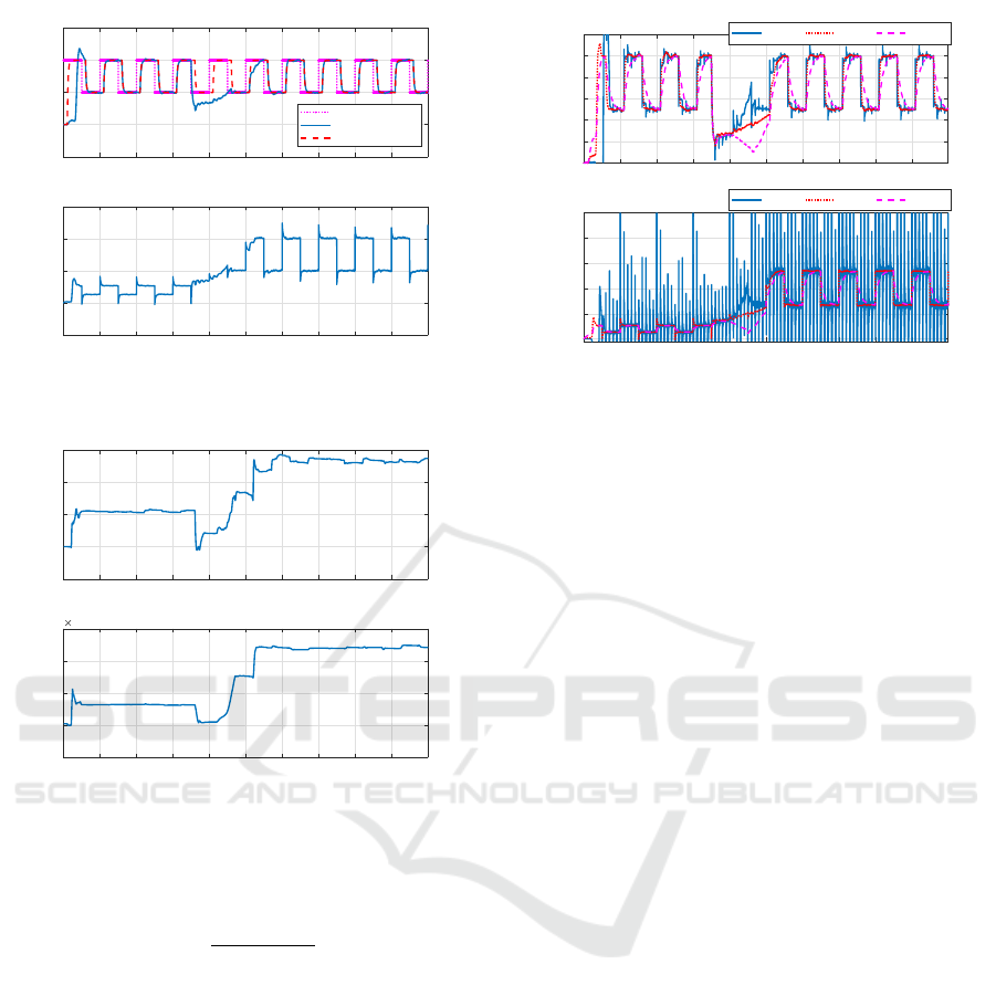
Figure 7: Experimental result by using the proposed
method.
Figure 8: Trajectories of the PI gains corresponding to Fig.
7.
A mismatch between the controller and the controlled
object is considered to cause deterioration. Although
the experimental system is a high-order system, the
controller is designed for a first-order controlled ob-
ject.
At last, the role of the predictive term is consid-
ered. the predictive PI control low is as follows:
u(t) =
K
P
+
K
I
∆
e(t) +
z
−1
K
pred
∆
(z
−d
− 1)u(t).
(45)
PID control low is also shown in follows:
u
PID
(t) =
K
P
+
K
I
∆
e(t) + K
D
∆e(t), (46)
where the third term is a derivative term and K
D
de-
notes a derivative gain. It is well-known that the
derivative term works like a brake. When PI gains
are large, sometimes large input is calculated by PI
Design of a Self-tuning Predictive PI Controller for Delay Systems based on the Augmented Output
677
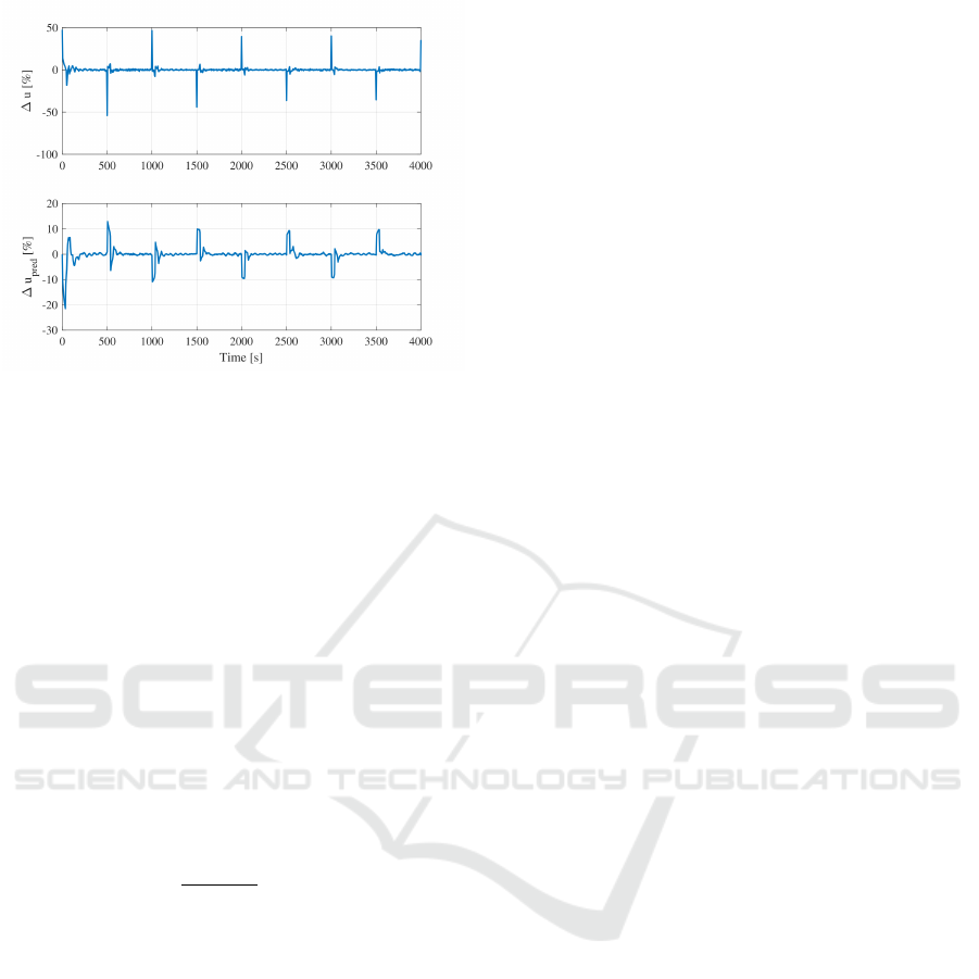
Figure 9: Comparison between ∆u(t) and ∆u
pred
(t).
terms and an overshoot is occurred. In contrast, the
derivative term predicts a future error and calculate
an input which reduces the overshoot based on the es-
timated error. The derivative term predicts a future
error under the assumption that the error is a propor-
tional function. However, the assumption is unrealis-
tic, and a large derivative gain sometimes causes prob-
lems. In contrast, the predictive term of the predictive
PI controller is based on a Smith predictor when a
controlled object is first order. Therefore, the predic-
tive PI controller employs more advanced prediction
than the PID controller although the predictive and
derivative terms have the same role.
Next, the consideration above is checked using the
experimental result. The input signal calculated by
the predictive term is defined as:
u
pred
(t) =
z
−1
K
pred
∆
(z
−d
− 1)u(t). (47)
Fig. 9 shows a comparison between ∆u(t) and
∆u
pred
(t). According to Fig. 9, the prediction term
worked like a brake. For example, ∆u(t) was about
−50 at 1505 second to lower the temperature. In con-
trast, ∆u
pred
(t) was about 10 between 1505 and 1535
seconds. The 30 seconds between 1505 and 1535
mean the estimated dead-time, and the predictive term
tried to suppress a large input signal in the period.
Thus, the control result shows that the predictive term
has the same role as the derivative term.
6 CONCLUSIONS
In this paper, a discrete-time predictive PI controller
has been discussed, and a data-driven self-tuning de-
sign method has also been proposed. Features of the
proposed controller are summarized as follows:
• The proposed controller can realize fast rise time
for a system with long dead-time.
• Any system model is not required to calculate PI
gains.
• Only PI gains are tuned in an on-line manner.
The proposed control scheme has been evaluated by
some numerical and experimental examples. In par-
ticular, the role of the predictive term included in the
proposed controller has been mentioned using the ex-
perimental example.
REFERENCES
Airikka, P. (2014). Robust predictive pi controller tuning.
IFAC Proceedings Volumes, 47(3):9301 – 9306. 19th
IFAC World Congress.
Ashida, Y., Hayashi, K., Wakitani, S., and Yamamoto, T.
(2016). A novel approach in designing pid controllers
using closed-loop data. In 2016 American Control
Conference (ACC), pages 5308–5313.
Ashida, Y., Wakitani, S., and Yamamoto, T. (2017). Design
of an implicit self-tuning pid controller based on the
generalized output. In Proc. of the 20th IFAC World
Congress, pages 14511 – 14516.
Ashida, Y., Wakitani, S., and Yamamoto, T. (2019). De-
sign of a data-driven pi controller. In Proc. of the
2020 International Conference on Artificial Life and
Robotics.
Astrom, K. and Hagglund, T. (2005). Advanced PID Con-
trol. International Society of Automation, North Car-
olina.
Berner, J., Soltesz, K., Hagglund, T., and Astrom, K.
(2018). An experimental comparison of pid auto-
tuners. Control Engineering Practice, 73:124–1133.
Bialkowski, W. (1993). Dreams versus reality: a view from
both sides of the gap: manufacturing excellence with
come only through engineering excellence. Pulp &
Paper Canada, 94:19–27.
Campestrini, L., Eckhard, D., Chia, L. A., and Boeira, E.
(2016). Unbiased mimo vrft with application to pro-
cess control. Journal of Process Control, 39:35 – 49.
Campi, M., Lecchini, A., and Savaresi, S. (2002). Virtual
reference feedback tuning: a direct method for the de-
sign of feedback controllers. Automatica, 38(8):1337
– 1346.
Gallego, A. J., Merello, G. M., Berenguel, M., and Cama-
choa, E. F. (2019). Gain-scheduling model predictive
control of a fresnel collector field. Control Engineer-
ing Practice, 82:1–13.
Goodwin, G. C. and Sin, K. S. (1984). Adaptive Filtering
Prediction and Control. Prentice-Hall, Upper Saddle
River.
Hagglund, T. (1992). A predictive pi controller for pro-
cesses with long dead times. IEEE Control Systems
Magazine, 12(1):57–60.
ICINCO 2019 - 16th International Conference on Informatics in Control, Automation and Robotics
678

Hassan, S. M., Ibrahim, R., Saad, N., Asirvadam, V. S., and
Chung, T. D. (2016). Predictive pi controller for wire-
less control system with variable network delay and
disturbance. In 2016 2nd IEEE International Sym-
posium on Robotics and Manufacturing Automation
(ROMA), pages 1–6.
Hjalmarsson, H., Gevers, M., Gunnarsson, S., and Lequin,
O. (1998). Iterative feedback tuning: theory and appli-
cations. IEEE Control Systems Magazine, 18(4):26–
41.
Ingimundarson, A. and Hagglund, T. (2001). Robust tuning
procedures of dead-time compensating controllers.
Control Engineering Practice, 9:1195–1208.
Kaneko, O. (2015). Fictitious reference iterative tuning of
internal model controllers for a class of nonlinear sys-
tems. In 2015 IEEE Conference on Control Applica-
tions (CCA), pages 88–94.
Rawlings, J. B. and Mayne, D. Q. (2009). Model Predic-
tive Control Theory and Design. Nob Hill Publishing,
Madison.
Sanz, R., Garcia, P., and Albertos, P. (2018). A generalized
smith predictor for unstable time-delay siso systems.
ISA Transactions, 72:197–204.
Soma, S., Kaneko, O., and Fujii, T. (2004). A new approach
to parameter tuning of controllers by using one-shot
experimental data (in japanese). Transactions of the
Institute of Systems, Control and Information Engi-
neers, 17(12):528–536.
Sun, L., Li, D., and Lee, K. Y. (2016). Optimal disturbance
rejection for pi controller with constraints on relative
delay margin. ISA Transactions, 63:103–111.
Wang, Y. and Ma, G. (2015). Fault-tolerant control of lin-
ear multivariable controllers using iterative feedback
tuning. International Journal of Adaptive Control and
Signal Processing, 29(4):457–472.
Design of a Self-tuning Predictive PI Controller for Delay Systems based on the Augmented Output
679
