Control Strategies for an Octopus-like Soft Manipulator

Simone Cacace

, Anna Chiara Lai

2 a

and Paola Loreti

Dipartimento di Matematica e Fisica, Universit

a degli Studi Roma Tre, Largo S. Murialdo, 1,

00154 Rome, Italy

Dipartimento di Scienze di Base e Applicate per l’Ingegneria, Sapienza Universit

a di Roma, Via A. Scarpa, 16, 00161

Rome, Italy

Keywords:

Soft Manipulators, Octopus Arm, Control Strategies.

Abstract:

We investigate a reachability control problem for a soft manipulator inspired to an octopus arm. Cases mod-

elling mechanical breakdowns of the actuators are treated in detail: we explicitly characterize the equilibria,

and we provide numerical simulations of optimal control strategies.

1 INTRODUCTION

In this paper we investigate a control theoretical

framework for a soft manipulator model, and we

present related numerical simulations. Our model al-

lows to deal with the case in which only a portion

of the manipulator is controlled, while the remain-

ing part of the device is driven by internal reaction

forces only. This scenario includes mechanical break-

downs, or a voluntary deactivation for energy saving

purposes: its investigation is one of the main novel-

ties also with respect to (Cacace et al., 2018), where

the model is originally introduced.

Soft manipulators attracted the interest of re-

searchers due to their ability to adapt to constrained

enviroments, and their potential suitability for human-

robot interactions (Rus and Tolley, 2015; Laschi and

Cianchetti, 2014). Starting from the ﬁrst works on

hyper-redundant manipulators (Chirikjian and Bur-

dick, 1990; Chirikjian and Burdick, 1995), the chal-

lenging motion planning of tentacle-like soft manipu-

lators was attacked by several points of view: among

many others, we refer to (Jones and Walker, 2006) for

the study of the kinematics, to (Kazakidi et al., 2015;

Kang et al., 2011) for a discrete dynamical model, to

(Lai and Loreti, 2014; Lai and Loreti, 2012; Lai et al.,

2014) for a number theoretic approach, and to (Thu-

ruthel et al., 2016) for a machine learning implemen-

tation. To the best of our knowledge, the approach in

the present paper, based on optimal control theory of

PDEs (see for instance (Tr

oltzsch, 2010)), appears to

the be new.

https://orcid.org/0000-0003-2096-6753

Our device is modelled as an inextensible elastic

string with curvature constraints (i.e. the device can-

not bend over a ﬁxed threshold), and whose curvature

is pointwise forced by a control term, modelling an

angular elastic internal force. The resulting dynam-

ics is an evolutive controlled non-linear fourth order

partial differential equation, generalizing the classical

Euler-Bernoulli equation. At this stage of our inves-

tigation, we adopt some simpliﬁcations in the model

–we are dealing with a theoretical object, a fully re-

sponsive, noise free planar manipulator with inﬁnite

degrees of freedom– but this allows us to go into the

deep in the optimization process, by providing opti-

mal open loop controls for a reachability problem.

The paper is organized as follows. In Section 2

we introduce our model in full generality and we dis-

cuss some particular parameter settings. In Section

3 we investigate the problem of steering the tip of

the manipulator to a target point, while minimizing

a quadratic cost on the controls and the kinetic energy

at ﬁnal time of the manipulator. Section 4 contains

some numerical simulations and ﬁnally in Section 5

we draw our conclusions.

2 A CONTROL MODEL FOR A

SOFT MANIPULATOR

Our goal is to describe the dynamics of a soft manip-

ulator encompassing the following features:

- inextensibility: the manipulator can bend but not

stretch longitudinally.

Cacace, S., Lai, A. and Loreti, P.

Control Strategies for an Octopus-like Soft Manipulator.

DOI: 10.5220/0007921700820090

In Proceedings of the 16th International Conference on Informatics in Control, Automation and Robotics (ICINCO 2019), pages 82-90

ISBN: 978-989-758-380-3

Table 1: Exact constraint equations and related elastic po-

tentials derived from penalty method. The functions ν and

µ represent non-uniform elastic constants.

Constraint Constraint Penalization

equation elastic potential

Inextensibility |q

| = 1 None

Curvature |q

| ≤ ω ν(|q

− ω

)

Control q

× q

= ωu µ (ωu − q

× q

)

- bending moment: the soft structure of the device

resists to bending via an angular elastic potential.

- bending constraint: the manipulator cannot bend

over a ﬁxed threshold

- bending control: a time-varying, internal angular

elastic force is applied in order to pointwise force

the bending of the device.

From a morphological point of view, we regard the

manipulator as a three-dimensional body with an

axial symmetry, a non-uniform thickness and a ﬁxed

endpoint. In what follows we build up a system

of PDEs modelling the evolution of the curve on

the plane representing the symmetry axis. From a

physical point of view, such an axis is modelled as an

inextensible string, whose mass represents the mass

of the whole manipulator. Also bending constraints

(and controls) of the manipulator are projected on

the axis: they are identiﬁed by suitably weighted

curvature constraints. For instance, the bending

constraint is translated into forcing the curvature of

the axis under a ﬁxed (non-uniform) threshold ω; the

bending control is translated into forcing the signed

curvature to the quantity ωu, where u ∈ [−1,1] is

the control map. The relation between the original

three-dimensional problem and the projected one

is further discussed in Section 2.1 below. In what

follows, we focus on the symmetry axis evolu-

tion. The unknowns of our problem are the curve

q(s,t) : [0,1] × R

→ R

parametrizing the symmetry

axis of the manipulator in arclength coordinates, and

the associated inextensibility multiplier σ(s,t) ∈ R.

We denote by q

, q

partial derivatives in

space and time respectively. The quantity |q

represents the curvature of q, whereas the product

× q

:= q

· q

⊥

represents the signed curvature,

where the symbol q

⊥

denotes the counter-clockwise

orthogonal vector to q

. With these notations, we

summarize the constraints described above in Table

1. Note that also the bending moment allows for a de-

scription in terms of curvature constraints: imposing

the constraint |q

| = 0 by penalty method yields the

elastic potential ε|q

, for some elastic (constant in

time) function ε(s). We then consider the Lagrangian

L(q,σ) :=



ρ|q

−

σ(|q

− 1)

−



− ω



−

ε|q

−

µ(ωu − q

× q

)



ds ,

(1)

whose integral terms respectively represent the ki-

netic energy (ρ is the mass density), the exact inex-

tensibility constraint (σ is the Lagrange multiplier),

the curvature constraint, the bending moment, and the

curvature control. Equation of motions are then de-

rived via the least action principle – see (Cacace et al.,

2018). They result in the following system:



ρq



σq

− Hq

⊥



−



+ Hq

⊥



= 1

(2)

for (s,t) ∈ (0,1) × (0, T ). The map G :=

G[q,ν,ε, ω] = ε + ν



− ω



encompasses the

bending moment and the curvature constraint –

(·)

denotes the positive part. The map H :=

H[q,µ,u,ω] = µ (ωu − q

× q

) represents the control

term. Equation (2) is completed with suitable initial

data, and with the following boundary conditions for

t ∈ (0, T ):

- ﬁxed endpoint conditions:

(

q(0,t) = (0,0),

(0,t) = −(0,1)

- free endpoint conditions:











(1,t) = 0 (zero bending moment)

sss

(1,t) = 0 (zero shear stress)

σ(1,t) = 0 (zero tension boundary).

Note that the ﬁxed endpoint conditions are a mod-

elling choice, while the free endpoint conditions

follow from the stationarity conditions for the La-

grangian L.

For technical details on the derivation of the equa-

tions we refer to (Cacace et al., 2018).

2.1 Model Parameter Settings

We propose a parameter tuning in order to encompass,

in the one-dimensional model, the morphology of the

original three-dimensional manipulator. The key mor-

phological assumptions on the manipulator are the

following: axial symmetry and uniform mass density

. In particular, we assume that in its position at rest

(i.e. when its symmetry axis has uniformly zero cur-

vature) the manipulator is a solid of rotation, gener-

ated by the function d(s), s ∈ [0, 1]; we call Ω(s) the

Control Strategies for an Octopus-like Soft Manipulator

circle of radius d(s) representing the cross section of

the manipulator at the point s ∈ [0, 1] of its axis. Note

that d measures the thickness of the manipulator: in

octopus arm shaped manipulators, d is a decreasing

function. Choosing ρ(s) := πρ

d(s)

corresponds to

concentrate the mass of Ω(s) on its barycentre.

In our model, bending the manipulator determines

a compression/dilatation of the soft, elastic material

composing its body, for which we assume an uniform

yield point, i.e., the pointwise elastic forces must be

uniformly bounded by some F

max

in order to avoid

inelastic deformations. Now, due to the axial symme-

try, for every s ∈ [0,1], the maximal angular elastic

force in Ω(s) is attained on its boundary and it reads

F(s) = e|q

|d(s), where e is the elastic constant of

the material. Therefore the constraint F(s) ≤ F

max

equivalent to the curvature constraint |q

| ≤ ω, where

we set ω(s) = F

max

/(ed(s)).

2.1.1 On Mass Distributions with Exponential

Decay

In our numerical simulations, we assume ρ to have

an exponential decay. By the arguments above, this

choice is consistent with the case of three dimensional

structures whose thickness decays exponentially, and

it can be viewed as an interpolation of self-similar,

discrete structures (Lai et al., 2016a). In turn, self-

similarity assumption has several advantages from

both a practical and theoretical point of view. In-

deed, asking for a manipulator to be self-similar sim-

ply means to be composed by identical, rescaled mod-

ules. From a geometrical point of view, self-similarity

is a powerful assumption allowing, via fractal geome-

try techniques (Lai, 2012), for a detailed investigation

of inverse kinematics of the manipulator, see for in-

stance (Lai et al., 2016b).

2.2 Control Parameter Settings

We now show how to set the control parameters to

model a mechanical breakdown of the actuators.

We recall that the controlled elastic potential is

U[q,µ,u,ω] :=

µ(ωu − q

× q

)

and the associated elastic force is

F[q,µ, u, ω] := −(Hq

⊥

)

− (Hq

⊥

)

where H = µ(ωu − q

× q

). Clearly, to choose µ ≡ 0

is equivalent to neglect F, and it yields the uncon-

trolled dynamics:

ρq

= (σq

)

− (Gq

)

. (3)

More generally, to set µ(s) = 0 for s ∈ [s

] means

that the portion of q between [s

] is uncontrolled:

it evolves according to (3) with (time dependent, con-

trolled) boundary conditions in q(s

,t) and q(s

,t).

We conclude with some remarks on how the con-

trol deactivation affects the equilibria of the system.

A general formula for the equilibria of (2) is provided

in (Cacace et al., 2018): if µ(1) = µ

(1) = 0, then the

signed curvature κ := q

×q

of the (unique) equilib-

rium q of (2) is proportional to µ, precisely it satisﬁes

κ(s) = µ(s)

ω(s)u(s)

µ(s) + ε(s)

s ∈ (0,1).

In particular for µ ≡ 0 the equilibrium is given by

q(s,t) ≡ (0, −s) for all (s,t) ∈ [0, 1] × (0, T ). More

generally, if q is uncontrolled in [s

], i.e., µ(s) = 0

for all s ∈ [s

], then |q

| = |κ(s)| = 0, that is the

corresponding portion of the device at the equilibrium

is arranged in a straight line.

3 THE REACHABILITY

OPTIMAL CONTROL

PROBLEM

In this section we address the problem of steering

the tip of the device –i.e., q(1,t)– to a target point

∗

∈ R

, using controls that optimize accuracy, steadi-

ness and energy consumption. In the framework of

optimal control theory, this problem can be restated

as a constrained minimization of a cost functional in-

volving:

- the tip-target distance: we want the tip to reach

and remain close to the target;

- a quadratic cost on the controls, that is we want to

force the device –precisely, its symmetry axis– to

bend as least as possible.

- the kinetic energy of the whole manipulator at ﬁ-

nal time.

More formally, given q

∗

∈ R

and T, τ > 0, we want

to minimize the functional

J (q,u) =

2τ

|q(1,t)− q

∗

ds dt

ρ(s)|q

(s,T )|

ds,

(4)

among all the controls u : [0,1] × [0, T ] → [−1, 1], and

subject to the symmetry axis dynamics (2). The ﬁrst

two terms in J account respectively for the tip-target

distance and the quadratic cost on the controls, during

ICINCO 2019 - 16th International Conference on Informatics in Control, Automation and Robotics

all the evolution, whereas the last term corresponds to

the kinetic energy at the ﬁnal time T.

In what follows we give the ﬁrst order optimality

conditions for this control problem, that is we write

a system of PDEs, called the adjoint system, whose

unknowns are the stationary points (q,σ,u) of J (sub-

ject to the symmetry axis dynamics), and the related

multipliers ( ¯q,

σ) called the adjoint states. Roughly

speaking, if a control u

∗

is optimal, then the adjoint

system admits a solution of the form (q,σ,u

∗

, ¯q,

σ).

The adjoint system is composed by a variational in-

equality for the optimal control and four PDEs: two

of them describe the evolution of the adjoint states,

and two of them are simply the dynamics the system

is subject to, i.e., the equations of motion of the sym-

metry axis (2). Following (Cacace et al., 2018), the

adjoint states equations are:











ρ ¯q



σ ¯q

− H ¯q

⊥



−



G ¯q

+ H ¯q

⊥





σq

−

⊥



−



⊥



¯q

· q

= 0

(5)

for (s,t) ∈ (0,1) × (0,T ), where

- the maps G and H are deﬁned in Section 2.

- the maps

G and

H are the linearisations of G and

H, respectively. In particular

G[q, ¯q, ν, ω] = g[q, ν,ω]q

· ¯q

H[q, ¯q,µ] = µ ( ¯q

× q

+ q

× ¯q

) ,

where g[q, ν, ω] = 2ν1(|q

−ω

) and 1(·) stands

for the Heaviside function, i.e. 1(x) = 1 for x ≥ 0

and 1(x) = 0 otherwise.

System (5) is completed with the following ﬁnal and

boundary conditions, derived as well from the opti-

mality conditions:

- ﬁnal conditions:

¯q(s,T ) = −q

(s,T ), ¯q

(s,T ) = 0

for s ∈ (0, 1). We point out that initial conditions

for q are replaced in the adjoint system with ﬁnal

conditions for ¯q: this is a quite fair consequence of

the fact that the optimization process takes into ac-

count the dynamics on the whole timeline (0,T ).

- ﬁxed endpoint boundary conditions:

¯q(0,t) = 0, ¯q

(0,t) = 0

for t ∈ (0,T ) – remark the symmetry with the

ﬁxed endpoint conditions on q;

- free endpoint boundary conditions:











¯q

(1,t) = 0

¯q

sss

(1,t) =

τε



(q − q

∗

) · q

⊥



⊥

(1,t)

σ(1,t) = −

(q − q

∗

) · q

(1,t)

for t ∈ (0,T ). Note that we recover the zero bend-

ing moment condition, as for the free endpoint of

q. On the other hand, as one may expect, both the

shear stress condition on ¯q and the adjoint tension

boundary condition on

σ are affected by the fact

that the system is forced towards the target q

∗

Finally, the variational inequality for the control is

(u + ω

H[q, ¯q])(v − u)dsdt ≥ 0 . (6)

for every v : [0,1] × [0,T ] → [−1, 1], which provides,

in a weak sense, the variation of the functional J with

respect to u, subject to the constraint |u| ≤ 1.

4 NUMERICAL SIMULATIONS

The optimal control problem discussed in Section 3

is approached in two phases. At a ﬁrst stage we look

at a stationary optimal control problem, involving the

equilibria of the system (2). Then such stationary so-

lutions are used as initial guess for the original dy-

namic optimal control problem, i.e., for the numerical

solution of the system composed by (2), (5) and (6).

4.1 Stationary Optimal Control

Problem

First of all we remark that if (q, σ) is an equilib-

rium for the symmetry axis equation (2) and if µ(1) =

(1) = 0, then q is the solution of the following sec-

ond order ODE:











µω

µ + ε

⊥

in (0,1)

= 1 in (0,1)

q(0) = (0,0)

(0) = −(0,1).

(7)

The stationary optimal control problem is the follow-

ing

min



ds +

2τ

|q(1) − q

∗



, (8)

subject to (7) and to |u| ≤ 1. Note that the above cost

functional is the stationary version of J : a quadratic

cost on the controls and a tip-target distance are still

involved, whereas time integrals and time-dependent

terms as the kinetic energy are clearly neglected. Us-

ing the ﬁrst two equations of (7), we have |q

| =

ω|u|,

where

ω := µω/(µ + ε). Therefore we can get rid of

the dependence from u in (7) and look for the solu-

Control Strategies for an Octopus-like Soft Manipulator

Table 2: Global parameter settings.

Parameter description Setting

mass distribution ρ(s) = exp(−s)

bending moment ε(s) = 10

−3

(1 − 0.9s)

curvature constraint ν(s) = 10

−3

(1 − 0.09s)

penalty

curvature control µ(s) = (1 − s)e

−0.1

1−s

penalty

curvature constraint ω(s) = 3π(1 + s

)

target point q

∗

= (0.3563,−0.4423)

target penalty τ = 10

−4

Discretization step ∆

= 0.05

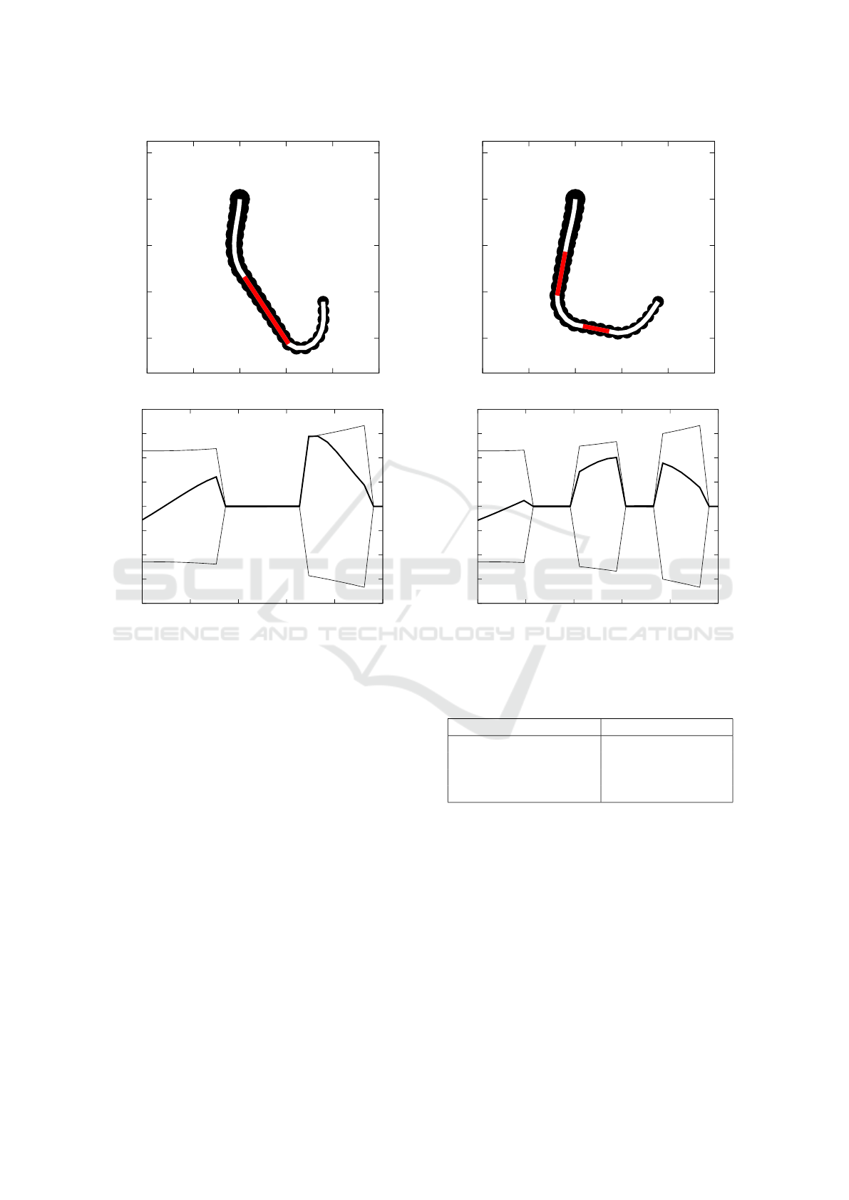
Table 3: Control deactivation settings related to µ

Test Control deactivation region

Test 1 I =

Test 2 I = [0.35, 0.65]

Test 3 I = [0.25, 0.4] ∪ [0.6,0.75]

tions of the following Euler elastica’s like problem:

min



(0,1)\I

ds +

2τ

|q(1) − q

∗



subject to











= 1 in (0,1)

| ≤

ω in (0,1)

q(0) = (0,0)

(0) = −(0,−1),

(9)

where we set I := {s ∈ (0, 1) | µ(s) = 0}. In other

words we are looking for the curve q –with length

1 and curvature bounded by

ω– minimizing the total

curvature and the distance of its tip from q

∗

. Dot-

multiplying by q

⊥

both sides of the ﬁrst equation of

(7), we obtain that the optimal control for the original

stationary problem (8) is then given by

u(s) =

(

(s)·q

⊥

(s)

ω(s)

if µ(s) 6= 0,

0 otherwise.

(10)

Note that in (Cacace et al., 2018) we assumed µ >

0 in (0,1). Here we also consider the case µ(s) =

0. As a matter of fact, for µ(s) = 0, the dynamics

and its equilibria are independent from u(s): it can be

arbitrarily chosen. The particular choice u(s) = 0 in

I allows the cost functional (8) to be consistent also

with the case of uncontrolled regions.

To numerically solve (9) we encompass the con-

straints |q

| = 1 and |q

| ≤

ω via an augmented La-

grangian method, and we discretize it with a ﬁnite dif-

ference scheme. The non-linear terms of the resulting

discrete system of equations are treated via a quasi

Newton’s method. Parameters settings are reported in

Table 2.

-0.6

-0.4

-0.2

0.2

-0.4 -0.2 0 0.2 0.4 0.6

(a)

-20

-15

-10

-5

0 0.2 0.4 0.6 0.8 1

(b)

Figure 1: In (a) the solution q of Test 1, in (b) the related

signed curvature κ(s) (bold line) and curvature constraints

ω (thin lines).

We investigate the problem in three scenarios, see

Table 3: in the ﬁrst we assume that µ is positive in

(0,1), in the second and third experiment we neglect

µ in some sub-intervals of (0,1). The latter cases rep-

resent situations in which we cannot control a portion

of the device – see Section 2.2. In particular, for a

given I ⊂ (0,1), we employ the following curvature

control penalty parameter

(s) =

(

0 if s ∈ I

µ(s) otherwise.

In Figure 1 we report the results of Test 1 –see

Table 3. In Figure 2 and 3 we show the results of Test

2 and Test 3, respectively. In these cases the controls

are in-actuated in a subset of (0,1): the corresponding

regions are depicted in red. The particular choice of

∗

allows for it to be reached in all these three cases,

but clearly, with different optimal solutions.

ICINCO 2019 - 16th International Conference on Informatics in Control, Automation and Robotics

-0.6

-0.4

-0.2

0.2

-0.4 -0.2 0 0.2 0.4 0.6

(a)

-20

-15

-10

-5

0 0.2 0.4 0.6 0.8 1

(b)

Figure 2: In (a) the solution q of Test 2, in (b) the related

signed curvature κ(s) (bold line) and curvature constraints

ω (thin lines).

4.2 Dynamic Optimal Control Problem

We address the minimization of the cost functional J

subject to a dissipative version of the dynamical sys-

tem (2):

ρq



σq

− Hq

⊥



−



+ Hq

⊥



− βq

− γq

sssst

(11)

In particular, the term −βq

represents an environ-

mental viscous friction proportional to the velocity;

the term −γq

sssst

an internal viscous friction, propor-

tional to the change in time of the curvature. This

implies that if we plug in (11) the optimal stationary

(constant in time) control u given in Equation (10),

then the system converges as T → +∞ to the optimal

stationary equilibrium q described in Section 4.1 - see

Equation (7). Here we look for time-varying optimal

controls, i.e., for solutions u

∗

of the dynamic optimal

control problem described in Section 3. The adjoint

-0.6

-0.4

-0.2

0.2

-0.4 -0.2 0 0.2 0.4 0.6

(a)

-20

-15

-10

-5

0 0.2 0.4 0.6 0.8 1

(b)

Figure 3: In (a) the solution q of Test 3, in (b) the related

signed curvature κ(s) (bold line) and curvature constraints

ω (thin lines).

Table 4: Dynamic parameter settings.

Parameter description Setting

Environmental friction β(s) = β(s) := 2 − s

Internal friction γ(s) := 10

−6

(2 − s)

Final time T = 2

Time discretization step ∆

= 0.001

states equations in the dissipative version read:











ρ ¯q



σ ¯q

− H ¯q

⊥



−



G ¯q

+ H ¯q

⊥





σq

−

⊥



−



⊥



+β ¯q

+ γ ¯q

sssst

¯q

· q

= 0

(12)

for (s,t) ∈ (0,1) × (0,T ).

The adjoint system composed by (11), (12) and

(6) can be discretized using a standard ﬁnite differ-

ence scheme in space-time, then solved by an adjoint-

based gradient descent method. The key idea is the

following: starting from an initial guess u given by the

Control Strategies for an Octopus-like Soft Manipulator

100

200

300

400

500

600

0 0.5 1 1.5 2

(a)

100

200

300

400

500

600

0 0.5 1 1.5 2

(b)

Figure 4: Time evolution of target energy J

∗

for the static

(a) and dynamic (b) optimal control.

stationary optimal control, we ﬁrst solve the equation

of motion (11) forward in time. Then the solution-

control triplet (q, σ,u) is plugged into (12) which is

solved backward in time. Finally, we use the vector

(q,σ, u, ¯q,

σ) in (6) to update the value of the u. The

procedure is iterated up to convergence on the control.

We assume that µ(s) = 0 in a subinterval I =

[0.35,0.65] of (0,1) – this choice corresponding to

Test 2 in Section 4.1, see Table 3 and Figure 1. In

other words, we are modelling the scenario in which

approximately one third of the central actuators of the

device are out of order. The parameters related to

the dynamical aspects, in particular those involved by

friction forces and time discretization are reported in

Table 4. The other parameters are set as in Section

4.1, see Table 2.

We compare the performances of optimal station-

ary and dynamic controls in terms of the evolution

of the three components of our integral cost: the

tip-target distance, the control energy and the kinetic

energy.

In Figure 4 we plot the function

∗

(t) := |q(1,t)− q

∗

representing the tip-target distance at time t ∈ [0,2],

in both cases of statically and dynamically optimized

controls. More precisely, in Figure 4(a) we plugged in

the system (11) a constant in time control u

, that we

call static optimal control, given by the solution of the

stationary control problem (8). We then considered

the resulting trajectory q(s,t) and measured the tip-

target distance J

∗

(t). In Figure 4(b) we see the tip-

target distance of the trajectory q obtained by numer-

ically solving the adjoint system, that is the trajectory

corresponding to a time-dependent optimal control u

that we call in the sequel dynamic optimal control.

In agreement with the theoretical setting, in particu-

lar with the strong dependence of the cost functional

J on the tip-target distance (see also the value for the

weight τ in Table 2), the dynamical optimization pro-

cess yields, up to some oscillations, a much lower

∗

(t) than the stationary case. We also remark the

damping of the oscillations of J

∗

(t) in the dynamical

case: this conﬁrms that the dynamical optimization

process tends to reach and stay close to the target as

soon as possible.

In Figure 5 we plot the function

(t) :=

(t)ds

representing the quadratic cost on the controls at time

t ∈ [0,2]. In the case of static controls, J

(t) is con-

stant by construction. The dynamic optimal controls

(t) are on average smaller than J

(t): this implies

that the dynamical optimization process actually re-

duces the total cost of the controls

(t)dt

with respect to the stationary optimization. Also note

that the dynamic optimal control u

yields a large

variation of its cost J

(t) at the beginning of the evo-

lution, while stabilizing it around the static control

cost J

(t) in a second time. This implies that the op-

timization process tends to concentrate the variation

of controls at the beginning, while the second part of

the evolution is demanded to small adjustments, con-

ﬁrming what we already remarked by looking at the

tip-target distance evolution.

Finally, in Figure 5 we plot the function

(t) :=

ρ(s)|q

(s,t)|

representing the kinetic energy of the whole axis at

time t ∈ [0,2] in the cases of stationary and dynamic

optimal controls. Note that the evolutions of the J

ICINCO 2019 - 16th International Conference on Informatics in Control, Automation and Robotics

0.0705

0.071

0.0715

0.072

0.0725

0.073

0.0735

0.074

0.0745

0.075

0 0.2 0.4 0.6 0.8 1 1.2 1.4 1.6 1.8 2

(a)

0.0705

0.071

0.0715

0.072

0.0725

0.073

0.0735

0.074

0.0745

0.075

0 0.2 0.4 0.6 0.8 1 1.2 1.4 1.6 1.8 2

(b)

Figure 5: Time evolution of control energy J

for the sta-

tionary (a) and dynamic (b) optimal control.

are comparable, but at ﬁnal time T , dynamical opti-

mal controls yield a kinetic energy J

(T ) lower than

the one associated to the stationary optimal controls.

This is consistent with the fact that the cost functional

J depends only on the kinetic energy at ﬁnal time.

Finally note that, since the system is converging to

an equilibrium due to frictional forces, J

(t) → 0 as

t → +∞: it is then reasonable to expect a larger time

frame to improve the performances of the kinetic en-

ergy in both dynamic and stationary cases. For the

dynamically controlled case only, steadiness can also

be traded with accuracy by increasing the weight of

the term J

(T ) in the functional J .

5 CONCLUSIONS

In this paper we addressed the optimal control of a

planar soft manipulator, modelled as an inextensible

elastic string with non-uniform mass, curvature con-

straints and curvature controls. Parameters are set in

order to encompass in the one-dimensional model the

0.5

1.5

2.5

3.5

0 0.2 0.4 0.6 0.8 1 1.2 1.4 1.6 1.8 2

(a)

0.5

1.5

2.5

3.5

0 0.2 0.4 0.6 0.8 1 1.2 1.4 1.6 1.8 2

(b)

Figure 6: Time evolution of kinetic energy J

for the static

(a) and dynamic (b) optimal control.

morphology of a three-dimensional manipulator. We

looked in particular to the case in which a part of the

device is uncontrolled and, consequently, driven only

by internal reaction forces. Optimal open loop con-

trols are obtained via a constrained minimization of

a cost functional in both the stationary and dynamic

case. Numerical simulations are provided in the spe-

cial case of partially actuated controls. They agree

with the theoretical control model.

A challenging open question is to ﬁnd alterna-

tive, not necessarily open loop, optimal strategies.

Then we plan to investigate other optimization tech-

niques, such as model predictive feedbacks and ma-

chine learning algorithms.

REFERENCES

Cacace, S., Lai, A. C., and Loreti, P. (2018). Modeling

and Optimal Control of an Octopus Tentacle. arXiv

e-prints, page arXiv:1811.08229.

Chirikjian, G. S. and Burdick, J. W. (1990). An obstacle

avoidance algorithm for hyper-redundant manipula-

Control Strategies for an Octopus-like Soft Manipulator

tors. In Proceedings., IEEE International Conference

on Robotics and Automation, pages 625–631. IEEE.

Chirikjian, G. S. and Burdick, J. W. (1995). The kinematics

of hyper-redundant robot locomotion. IEEE transac-

tions on robotics and automation, 11(6):781–793.

Jones, B. A. and Walker, I. D. (2006). Kinematics for mul-

tisection continuum robots. IEEE Transactions on

Robotics, 22(1):43–55.

Kang, R., Kazakidi, A., Guglielmino, E., Branson, D. T.,

Tsakiris, D. P., Ekaterinaris, J. A., and Caldwell,

D. G. (2011). Dynamic model of a hyper-redundant,

octopus-like manipulator for underwater applications.

In Intelligent Robots and Systems (IROS), 2011

IEEE/RSJ International Conference on, pages 4054–

4059. IEEE.

Kazakidi, A., Tsakiris, D. P., Angelidis, D., Sotiropoulos,

F., and Ekaterinaris, J. A. (2015). Cfd study of aquatic

thrust generation by an octopus-like arm under intense

prescribed deformations. 115:54–65.

Lai, A. C. (2012). Geometrical aspects of expansions

in complex bases. Acta Mathematica Hungarica,

136(4):275–300.

Lai, A. C. and Loreti, P. (2012). Discrete asymptotic reach-

ability via expansions in non-integer bases. In 2012 9-

th international conference on informatics in control,

automation and robotics (ICINCO), volume 2, pages

360–365. IEEE.

Lai, A. C. and Loreti, P. (2014). Robot’s hand and expan-

sions in non-integer bases. Discrete Mathematics &

Theoretical Computer Science, 16(1).

Lai, A. C., Loreti, P., and Vellucci, P. (2014). A model for

robotic hand based on ﬁbonacci sequence. In 2014

11th International Conference on Informatics in Con-

trol, Automation and Robotics (ICINCO), volume 2,

pages 577–584. IEEE.

Lai, A. C., Loreti, P., and Vellucci, P. (2016a). A continuous

ﬁbonacci model for robotic octopus arm. In 2016 Eu-

ropean Modelling Symposium (EMS), pages 99–103.

IEEE.

Lai, A. C., Loreti, P., and Vellucci, P. (2016b). A ﬁbonacci

control system with application to hyper-redundant

manipulators. Mathematics of Control, Signals, and

Systems, 28(2):15.

Laschi, C. and Cianchetti, M. (2014). Soft robotics: new

perspectives for robot bodyware and control. Frontiers

in bioengineering and biotechnology, 2:3.

Rus, D. and Tolley, M. T. (2015). Design, fabrication and

control of soft robots. Nature, 521(7553):467–475.

Thuruthel, T., Falotico, E., Cianchetti, M., Renda, F., and

Laschi, C. (2016). Learning global inverse statics so-

lution for a redundant soft robot. In Proceedings of

the 13th International Conference on Informatics in

Control, Automation and Robotics, volume 2, pages

303–310.

oltzsch, F. (2010). Optimal control of partial differential

equations: theory, methods, and applications, volume

112. American Mathematical Soc.

ICINCO 2019 - 16th International Conference on Informatics in Control, Automation and Robotics