An Improved APFM for Autonomous Navigation and Obstacle

Avoidance of USVs

Xiaohui Zhu

1,2,3 a

, Yong Yue

, Hao Ding

3,4

, Shunda Wu

, MingSheng Li

and Yawei Hu

Department of Computer Science and Software Engineering, Xi’an Jiaotong-Liverpool University,

Suzhou, Jiangsu Province, 215123, P. R. China

Department of Computer Science, University of Liverpool, Liverpool, L69 3BX, U.K.

School of Information Science and Technology, Nantong University, Nantong, Jiangsu Province, 226019, P. R. China

Nantong Research Institute for Advanced Communication Technologies, Nantong, Jiangsu Province, 226019, P. R. China

Keywords:

Autonomous Navigation, Obstacle Avoidance, Improved APFM, USVs, Water Quality Monitoring.

Abstract:

Unmanned surface vehicles (USVs) are getting more and more attention in recent years. Autonomous navi-

gation and obstacle avoidance is one of the most important functions for USVs. In this paper, we proposed

an improved angle potential ﬁeld method (APFM) for USVs. A reversed obstacle avoidance algorithm was

proposed to control the steering of USVs in tight spaces. In addition, a multi-position navigation route plan-

ning was also achieved. Simulation results in MATLAB show that the improved APFM can guide the USV

to autonomously navigate and avoid obstacles around the USV during navigation. We applied the algorithm

to a real USV, which is designed for water quality monitoring and tested in a real river system. Experimental

results show that the improved APFM can successfully guide the USV to navigate based on the predeﬁned

navigation route while detecting both static and dynamic obstacles and avoiding collisions.

1 INTRODUCTION

With the development of sensor technology, mobile

network, autonomous navigation and artiﬁcial intel-

ligence (AI), unmanned surface vehicles (USVs) are

getting more and more attention in scientiﬁc research

(Liu et al., 2017), environmental missions (Polvara

et al., 2018a) , military operations and civilian ap-

plications (Liu et al., 2016). Many countries, espe-

cially those with vast water resources are vigorously

developing USVs (Zhou et al., 2015). US Naval Un-

dersea Warfare Center developed the Spartan Scout

USV, an advanced concept technology demonstration

in 2002 (Maguer et al., 2005). In Japan, Yamaha

developed two USVs, the Unmanned Marine Ve-

hicle High-Speed UMV-H and the Unmanned Ma-

rine Vehicle Ocean type UMV-O for monitoring bio-

geo-chemical parameters of oceans and atmosphere

(Enderle et al., 2004). The Portuguese Dynamical

Systems and Ocean Robotics Laboratory developed

several marine robotic vessels(Bertram, 2008). Ac-

cording to practical applications and requirements,

USVs have various appearances such as rigid inﬂat-

https://orcid.org/0000-0003-1024-5442

able hulls, kayaks, catamarans and trimarans (Naeem

et al., 2008; Peng et al., 2009). Due to catamaran’s

stability in heavy-weather situations and its ample

space for setting additional water quality monitoring

devices, it is widely used in environmental monitor-

ing.

Generally, USVs usually consist of three main

modules: data acquisition, path planning and naviga-

tion control. Many researchers have proposed vari-

ous algorithms for autonomous navigation and colli-

sion avoidance (Li et al., 2017; Wang et al., 2011;

Zhang et al., 2014a). Artiﬁcial potential ﬁeld method

was a real-time obstacle avoidance approach (Khatib,

1986a). It use attractive force to allow robots to

reach the destination and use repulsion force to keep

robots away from obstacles. The resultant of these

two forces can guide the robot to avoid obstacles dur-

ing the navigation. The approach is widely used due

to its advantages of simplicity and small computing

requirement. However, it also has a disadvantage of

having local optimal solutions. Borenstein proposed

a vector ﬁeld histogram(VFH) algorithm to achieve

obstacle avoidance for fast mobile robots in cluttered

environments (Borenstein and Koren, 1990). It uses a

two-dimensional Cartesian histogram grid as a world

Zhu, X., Yue, Y., Ding, H., Wu, S., Li, M. and Hu, Y.

An Improved APFM for Autonomous Navigation and Obstacle Avoidance of USVs.

DOI: 10.5220/0007922904010408

In Proceedings of the 16th International Conference on Informatics in Control, Automation and Robotics (ICINCO 2019), pages 401-408

ISBN: 978-989-758-380-3

401

model. The VFH algorithm is efﬁcient and robust.

However, the size of grid cells is highly related to the

computing performance. The smaller the grid cell,

the clearer the environmental information is drawn,

but the amount of computational time and storage

space will increase exponentially. With the develop-

ment of artiﬁcial intelligence (AI), AI algorithms such

as neural network and particle swarm optimization

were also used for autonomous navigation (Polvara

et al., 2018b; Zhang et al., 2014b). However, AI al-

gorithms usually need much more computational re-

sources. Due to the constrained electric energy and

computing resources on small USVs, it is not always

available for small USVs. The angle potential ﬁeld

method (APFM) can guide mobile robots to reach the

destination by a combined force from obstacles and

the destination (Li and He, 2006).

In this paper, we review the fundamental concept

of APFM in Section II. Section III introduces the im-

proved APFM according to the particular requirement

of USVs. We simulate the improved APFM in MAT-

LAB to analysis the correctness and performance of

our algorithm in Section IV. We apply the algorithm

to a real USV and test in a lake in Section V. Finally,

we make a conclusion in Section VI.

2 ANGLE POTENTIAL FIELD

METHOD

The angle potential ﬁeld method (APFM) was pro-

posed for outdoor mobile robots in 2006 (Li and He,

2006). The APFM is based on an artiﬁcial poten-

tial ﬁeld concept (Khatib, 1986b). The main idea of

APFM is: each obstacle around the robot produces a

resistance to the robot, and the target point produces

an attraction to the robot. The accessibility of each

angle for the robot is determined by the ratio of at-

traction and resistance. The angle with maximal ac-

cessibility is the heading for the robot.

2.1 Resistance of Obstacles

The resistance to a robot is produced by surrounding

obstacles. When the linear distance D

between an

obstacle and the robot is decreased, the resistance is

increased. Otherwise, the resistance is decreased. We

assume D

is the minimal safety lateral distance be-

tween the robot and an obstacle for the robot to safely

pass through the obstacle. The D

is deﬁned as fol-

lows.

W (1)

Figure 1: Risk collision area of an obstacle in the robot ﬁxed

coordinate frame.

where W is the width of the robot, K

is a coefﬁcient

to extend the safety lateral distance between the robot

and an obstacle, and K

≥ 1.

We let θ be the angle of an obstacle in the robot

ﬁxed coordinate frame. Figure 1 shows the risk colli-

sion area of an obstacle to the robot in navigation. The

risk angle φ for the robot is deﬁned by the following

equation.

φ = argsin(

) (2)

Equation 2 means that if the heading of the robot is

within the angle φ, the robot will collide with the ob-

stacle. As we know that the robot may pass through

the obstacle from the right or left side, the collision

angle ϕ for the robot is shown as follows.

θ − φ ≤ ϕ ≤ θ + φ (3)

Let D

min

be the minimum safety linear distance

between an obstacle and the robot, D

max

be the max-

imum distance of obstacle detection, K

(θ,ϕ) be the

resistance of an obstacle at angle θ to the robot at an-

gle ϕ. We let K

(θ,ϕ) be a small constant when the

distance D

is larger than D

max

. if D

is smaller than

min

, it means that the robot will collide with the ob-

stacle and we let K

(θ,ϕ) be a inﬁnite value. Oth-

erwise, K

(θ,ϕ) is inversely proportional to the dif-

ference between D

and D

min

. Equation 4 means that

when the heading of the robot is not within the colli-

sion angle, we do not need to calculate the resistance

of the obstacle. Otherwise, we should calculate the

resistance K

(θ,ϕ) and there are three situations we

should consider based on the distance D

between the

robot and the obstacle.

ICINCO 2019 - 16th International Conference on Informatics in Control, Automation and Robotics

402

(θ,ϕ) =











0, i f ϕ > θ + φ or ϕ < θ − φ

+∞, i f D

< D

min

and θ − φ ≤ ϕ ≤ θ + φ

−D

min

, i f D

min

≤ D

max

and θ − φ ≤ ϕ ≤ θ + φ

max

−D

min

, i f D

> D

max

and θ − φ ≤ ϕ ≤ θ + φ

(4)

We let K

(ϕ) be the maximal resistance that all

obstacles in front of the robot at angle ϕ, which is

shown in Equation 5.

(ϕ) = max

ϕ∈[0 π]

(θ,ϕ)) (5)

2.2 Abstraction of Target Point

To guide the robot to move towards the target point,

we deﬁne an attraction K

(ϕ) for the target point at

angle ϕ as follows.

(ϕ) = cos(ϕ − θ

destinaton

) (6)

where θ

destinaton

is the angle of the target point and

ϕ is the heading of the robot. From Equation 6 we

know that when the deviation between the heading

of the robot and the destination is increased, the at-

traction K

(ϕ) is decreased. otherwise, K

(ϕ) will be

increased.

2.3 Pass Function

Based on the maximum resistance of obstacles around

the robot and the attraction of the destination to the

robot, we deﬁne a pass function K

(ϕ) as follows.

(ϕ) = max

ϕ∈[0 π]

(

(ϕ)

) (7)

We know from Equation 7 that the APFM tries to

ﬁnd a angle ϕ in [0 π] which has maximal value of

(ϕ). Then we should let the robot turn to that angle

and move forward. The process continues until the

robot reaches the target point.

3 IMPROVEMENT OF APFM

3.1 Issues in APFM

As we know that mobile robots are quite different

from USVs as follows. They should be carefully con-

sidered and solved before we can apply the APFM to

USVs.

• Mobile robots can accurately control or rapidly

change their moving speed on land. However, af-

fected by the wind and water ﬂows, it is difﬁcult

for USVs to strictly and immediately control and

change sailing speed.

• The steering operation of mobile robots is easy to

achieve. Constrained by steering angle of the rud-

der and the servo, the steering operation of USVs

needs much more time than mobile robots.

• When the distance between obstacles and the

robot is too small for the robot to turn, the original

APFM simply stops the robot. It is not acceptable

when we apply this algorithm to a real USV.

• The original APFM only considers the straight

path planning of a single position. To a real USV,

multi-position path planning has to be achieved.

• Further research shows that there is a potential is-

sue when there is no obstacle around the robot,

which means the resistance K

(ϕ) is 0. Equation

7 indicates that when K

(ϕ) is 0, we get a maxi-

mal K

(ϕ) no matter what the value of K

(ϕ) is. It

is unreasonable when there is more than one angle

which has a resistance of 0. Because in this situa-

tion, we still should select an angle which has the

largest attraction to the destination and drive the

USV toward this angle.

3.2 Improved APFM

According to the issues proposed above, we improve

the APFM as follows.

• Firstly, to simplify the speed and heading control

of the USV, we assume the USV has a stable speed

during navigation. It is easy to achieve in a real

application by controlling the ESC to provide sta-

ble power to the motor in the USV.

• Secondly, we use a Proportional-Integral-

Derivative (PID) controller to control the heading

of USV. The PID controller can continuously

adjust the heading of USV until it reaches the

desired heading.

• Thirdly, we propose a reversed obstacle avoidance

algorithm. When the distance between obstacles

and the USV is too small to turn the heading of

the USV, we let a position which is symmetric

with the actual target point of the USV regarding

the current position of the USV be the virtual tar-

get point and let the stern direction of the USV

An Improved APFM for Autonomous Navigation and Obstacle Avoidance of USVs

403

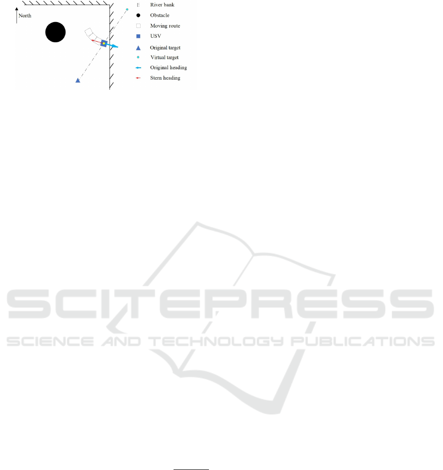
Figure 2: Reversed obstacle avoidance.

as a virtual heading. We apply the APFM again

based on the virtual target point and the heading

to guide the USV to move far away from obsta-

cles. Finally, We continue the navigation process

again to let the USV reach the real target point.

Figure 2 shows the procedure of the reversed ob-

stacle avoidance algorithm.

From ﬁgure 2 we know that the USV is at the cor-

ner of a river. Due to the closeness to the right

bank and its current heading, the USV cannot ﬁnd

a way to the original target point. In this situ-

ation, the reserved obstacle avoidance algorithm

will try to drive the USV back and head to the

virtual target point, which is symmetric with the

actual target point regarding the current position

of the USV. Finally, the heading of USV is turned

to the direction of the original target point, and the

navigation can be continued.

• Fourthly, we extend the single position path plan-

ning to multi-position path planning. Integrated

with the reversed obstacle avoidance algorithm,

At ﬁrst, we let the ﬁrst position as the current tar-

get point for the USV. When the USV reaches the

ﬁrst target, we let the subsequent positions as the

current target of the USV one by one. Finally, the

USV can reach the ﬁnal destination.

• Finally, to solve this potential issue when there is

no obstacle around the USV, we set the K

(ϕ) to a

very small constant when there is no resistance at

angle ϕ. we revise Equation 4 as follows. where

0 < ω < 1. It is easy to know that ω ∗

max

−D

min

is the smallest value in Equation 8, which means

there is no obstacle at the angle ϕ for the USV. So

the ﬁnal heading of the USV will be determined

by the attraction K

(ϕ) in Equations 6 and 7.

4 SIMULATIONS AND ANALYSIS

We assume the length and width of USV are both one

meter and the turning radius of the USV is 2.5 meters.

We deﬁne a 50*50 m square as a river area for the test.

In addition, we let the minimum safety linear distance

min

) between an obstacle and the USV be 2 meters,

the maximum distance (D

max

) for obstacle detection

be 8 meters and the minimal safety lateral distance

) between the USV and an obstacle be 1 meter.

We implemented the improved APFM in MATLAB

and considered several scenarios as follows.

4.1 Obstacle Detection and Avoidance

with Multiple Positions

The multi-position path planning is shown in Figure

3. We set a scenario with four navigation positions.

We let the ﬁrst position be the departure, and the

last position be the destination respectively. Figure 4

shows the navigation process. Because obstacles are

far away from the navigation route between the de-

parture position to the ﬁrst target position, the cruise

track between these two positions is a straight line.

Attracted by the second target position, the USV turns

right and moves towards the second target position.

Inﬂuenced by the resistance of the right bottom obsta-

cle, the USV slightly turns right again to avoid the ob-

stacle on its left side and reaches the second target po-

sition. With the attraction of the destination position

at the right top, the USV turns right again and moves

ahead to the destination. Affected by the resistance of

the central obstacle, the USV starts to turn left when

it moves close to the central obstacle. However, at-

tracted by the destination, the USV turns slightly right

but still have enough safety distance from the obsta-

cle. Finally, it reaches the destination.

4.2 Reversed Obstacle Avoidance

between Two Positions

In this simulation, we set the departure position at the

right top, which is very close to the right bank of the

river and the destination position at the left bottom.

Similar to the previous simulation, there is an obsta-

cle between the departure and destination positions.

Figure 5 shows the simulation result.

The purple ellipse is the area where the reversed

obstacle avoidance algorithm works. Figure 6 shows

the detailed process of reversed obstacle avoidance.

The cruise track of the USV is the blue rectangles.

The grey rectangles represent the brake track of the

USV when it is close to the right border. The red rect-

angles are the cruise track when the reversed obstacle

avoidance algorithm works.

Constrained by the minimum turning radius of

the USV, during the turning process, the USV is too

close to the right border and cannot turn. The USV

is stopped when the distance between the USV and

the right border is smaller than the minimum safety

ICINCO 2019 - 16th International Conference on Informatics in Control, Automation and Robotics

404

(θ,ϕ) =











ω ∗

max

−D

min

, i f ϕ > θ + φ or ϕ < θ − φ

+∞, i f D

< D

min

and θ − φ ≤ ϕ ≤ θ + φ

−D

min

, i f D

min

≤ D

max

and θ − φ ≤ ϕ ≤ θ + φ

max

−D

min

, i f D

> D

max

and θ − φ ≤ ϕ ≤ θ + φ

(8)

Figure 3: Multi-position path planning.

Figure 4: Obstacle detection and avoidance with multiple

positions.

distance D

min

. Then, the reversed obstacle avoidance

algorithm guides the USV to go backwards and turn

right. As a result, the USV leaves far away from the

right border of the river and turns the heading to the

destination position. Finally, the USV has enough

turning radius and is guided by the improved APFM

to avoid obstacles and reaches the destination position

at the left bottom.

4.3 Obstacle Detection and Avoidance

with Moving Obstacles

We simulate a scenario with moving obstacles. We

add a referential USV with a speed of 1m/s as a mov-

Figure 5: Reversed obstacle avoidance between two posi-

tions.

Figure 6: Enlarged image for the process of reversed obsta-

cle avoidance.

ing obstacle and assume it can only detect static ob-

stacles. The referential USV moves from the left po-

sition towards the right bottom position. We use red

rectangles to identify the cruise track of the referen-

tial USV. Figure 7 demonstrates the process of mov-

ing obstacle detection and avoidance when two USVs

meet each other. We ﬁnd that when two USVs are ap-

proaching, the referential USV cannot detect the ap-

proaching of another USV and does not change its

navigation route. However, the ﬁrst USV can de-

tect the referential USV, and the resistance from the

referential USV to the ﬁrst USV will be calculated.

Affected by another resistance from the obstacle and

the attraction from the immediate target position, the

USV slightly turns left to avoid the collision with the

referential USV and continues to go towards the des-

tination.

An Improved APFM for Autonomous Navigation and Obstacle Avoidance of USVs

405

Figure 7: Obstacle detection and avoidance with moving

obstacles.

5 USVS AND EXPERIMENTAL

RESULTS

5.1 Architecture of USVs

We developed a USV for water quality monitoring.

The main architecture of the USV is shown in Figure

8. During navigation, the USV uses a simple commer-

cial GPS receiver to continuously obtain its positions

from GPS satellites. The positioning accuracy of the

GPS receiver is 1.5 meters. An inertial measurement

unit (IMU) is used to obtain the USV’s heading and

acceleration in real time. In addition, the USV can de-

tect surrounding obstacles protruding from the water

surface using a single-line LIDAR. The detection dis-

tance of the LIDAR is 10 meters. All these data will

be input to the algorithm of autonomous navigation

and obstacle avoidance to guide the navigation of the

USV based on a predeﬁned navigation route. Water

quality sensors deployed under the USV body collect

water quality data at a regular interval. A 4G-based

data transfer unit (DTU) transfers water quality data

to the remote data center via the 4G mobile network

and the Internet. Finally, all the water quality data are

processed and saved in a database. Front end users

can use a web browser or an Android APP to query

and analyse water quality data respectively.

The USV is based on a catamaran. The stability,

payload capacity and ease of deck access make cata-

marans a compelling for USVs (Manley, 2008). Fig-

ure 9 shows the main components of the USV. All the

electronic devices such as the Raspberry Pi, battery,

DTU and GPS are all installed in the cabin. The wa-

ter quality monitoring sensors and a Doppler sensor

Figure 8: Architecture of USVs.

are deployed under the USV. Both live camera and

LIDAR are installed in the front of the USV.

5.2 Autonomous Navigation and

Obstacle Avoidance

5.2.1 Autonomous Navigation

The USV is tested in a small lake which is about 213

meters long and 196 meters wide. We select seven

positions using Google map to deﬁne a polygon and

zigzag navigation route respectively shown in Fig-

ures 10(a) and 10(b). The actual autonomous navi-

gation trajectory is shown in Figures 10(c) and 10(d).

Compared the actual navigation trajectory to the pre-

deﬁned navigation route we ﬁnd that the improved

APFM can guide the navigation of the USV based on

the predeﬁned navigation route. However, affected by

the wind and the accuracy of the GPS receiver, there

is a little deviation between the actual trajectory and

the predeﬁned route.

5.2.2 Obstacle Avoidance

We set another polygon route with ﬁve positions to

test the function of obstacle avoidance. We use two

balloons as static obstacles and one remote controlled

ship (RC ship) as a dynamic obstacle during the nav-

igation. The navigation route and the experimental

scenario are shown in Figure 11.

We use a RC ship to simulate a dynamic obstacle.

When the USV is navigating from the third position to

the fourth position, we remotely control the RC ship

move towards the USV to verify whether the USV can

detect the dynamic obstacle and avoid the collision

or not. From Figure 11(c) we ﬁnd that controlled by

the algorithm of autonomous navigation and obstacle

avoidance, the USV can autonomously navigate based

on the predeﬁned navigation route.

ICINCO 2019 - 16th International Conference on Informatics in Control, Automation and Robotics

406

(a) Components of the USV (b) Overall appearance of the USV

Figure 9: Main components of the USV.

(a) Polygon navigation route (b) Zigzag navigation route

Figure 10: Autonomous navigation without obstacles.

(a) Navigation route with obstacles (b) USV, balloons and RC ship (c) Actual track

Figure 11: Autonomous navigation with obstacles.

An Improved APFM for Autonomous Navigation and Obstacle Avoidance of USVs

407

6 CONCLUSIONS

We proposed an improved APFM for USVs. A re-

versed obstacle avoidance algorithm was developed

to improve the steering ability of the USV in tight

spaces. Integrated with multi-position path planning

approach and PID control, we simulated and tested

the improved APFM in MATLAB to validate the cor-

rectness and performance of our algorithm. Finally,

we applied our algorithm to a real USV and tested in

a real lake. Experimental results show that the USV

can autonomously navigate based on the predeﬁned

navigation route and avoid static and dynamic obsta-

cles.

ACKNOWLEDGEMENTS

This work was partly supported by the AI University

Research Centre (AI-URC) through XJTLU Key Pro-

gramme Special Fund (KSF-P-02), Natural Science

Foundation of Suzhou City (SYG201837), Natural

Science Foundation of Nantong City(JC2018075)and

Nantong University-Nantong Joint Research

Center for Intelligent Information Technology

(KFKT2017A06).

REFERENCES

Bertram, V. (2008). Unmanned surface vehicles-a survey.

Skibsteknisk Selskab, Copenhagen, Denmark, 1:1–14.

Borenstein, J. and Koren, Y. (1990). Real-time obstacle

avoidance for fast mobile robots in cluttered environ-

ments. In Proceedings., IEEE International Confer-

ence on Robotics and Automation, pages 572–577.

IEEE.

Enderle, B., Yanagihara, T., Suemori, M., Imai, H., and

Sato, A. (2004). Recent developments in a total

unmanned integration system. In Proc. AUVSI Un-

manned Systems Conference, volume 9.

Khatib, O. (1986a). Real-time obstacle avoidance for ma-

nipulators and mobile robots. In Autonomous robot

vehicles, pages 396–404. Springer.

Khatib, O. (1986b). Real-time obstacle avoidance for ma-

nipulators and mobile robots. In Autonomous robot

vehicles, pages 396–404. Springer.

Li, Y. and He, K. (2006). A novel obstacle avoidance and

navigation method for outdoor mobile robot based on

laser radar. Robot, 28(3):275–278.

Li, Z., Bachmayer, R., and Vardy, A. (2017). Vector ﬁeld

path following control for unmanned surface vehicles.

In OCEANS 2017-Aberdeen, pages 1–9. IEEE.

Liu, Y., Liu, W., Song, R., and Bucknall, R. (2017). Pre-

dictive navigation of unmanned surface vehicles in a

dynamic maritime environment when using the fast

marching method. International Journal of Adaptive

Control and Signal Processing, 31(4):464–488.

Liu, Z., Zhang, Y., Yu, X., and Yuan, C. (2016). Unmanned

surface vehicles: An overview of developments and

challenges. Annual Reviews in Control, 41:71–93.

Maguer, A., Gourmelon, D., Adatte, M., and Dabe, F.

(2005). Flash and/or ﬂash-s dipping sonars on spar-

tan unmanned surface vehicle (usv): A new asset for

littoral waters. In Turkish International Conference on

Acoustics.

Manley, J. E. (2008). Unmanned surface vehicles, 15 years

of development. In OCEANS 2008, pages 1–4. Ieee.

Naeem, W., Xu, T., Sutton, R., and Tiano, A. (2008). The

design of a navigation, guidance, and control system

for an unmanned surface vehicle for environmental

monitoring. Proceedings of the Institution of Mechan-

ical Engineers, Part M: Journal of Engineering for the

Maritime Environment, 222(2):67–79.

Peng, Y., Han, J.-d., and Huang, Q.-j. (2009). Adaptive ukf

based tracking control for unmanned trimaran vehi-

cles. International Journal of Innovative Computing,

Information and Control, 5(10):3505–3516.

Polvara, R., Sharma, S., Wan, J., Manning, A., and Sutton,

R. (2018a). Obstacle avoidance approaches for au-

tonomous navigation of unmanned surface vehicles.

The Journal of Navigation, 71(1):241–256.

Polvara, R., Sharma, S., Wan, J., Manning, A., and Sutton,

R. (2018b). Obstacle avoidance approaches for au-

tonomous navigation of unmanned surface vehicles.

The Journal of Navigation, 71(1):241–256.

Wang, H., Wei, Z., Wang, S., Ow, C. S., Ho, K. T., and

Feng, B. (2011). A vision-based obstacle detection

system for unmanned surface vehicle. In 2011 IEEE

5th International Conference on Robotics, Automation

and Mechatronics (RAM), pages 364–369. IEEE.

Zhang, R., Tang, P., Su, Y., Li, X., Yang, G., and Shi, C.

(2014a). An adaptive obstacle avoidance algorithm for

unmanned surface vehicle in complicated marine en-

vironments. IEEE/CAA Journal of Automatica Sinica,

1(4):385–396.

Zhang, R., Tang, P., Su, Y., Li, X., Yang, G., and Shi,

C. (2014b). An adaptive obstacle avoidance algo-

rithm for unmanned surface vehicle in complicated

marine environments. IEEE/CAA Journal of Automat-

ica Sinica, 1(4):385–396.

Zhou, X., Ling, L., Ma, J., Tian, H., Yan, Q., Bai, G., Liu,

S., and Dong, L. (2015). The design and application

of an unmanned surface vehicle powered by solar and

wind energy. In Power Electronics Systems and Ap-

plications (PESA), 2015 6th International Conference

on, pages 1–10. IEEE.

ICINCO 2019 - 16th International Conference on Informatics in Control, Automation and Robotics

408