
Wavelet Analysis based Stability Conditions of a Prediction Model
Ekaterina Sakrutina
a
V.A. Trapeznikov Institute of Control Sciences of Russian Academy of Science, 65 Profsoyuznaya, Moscow 117997, Russia
Keywords: Prediction Model, Multi-scale Wavelet Transform, Stability Conditions, Conditionless Prediction.
Abstract: Prediction models found a wide application in advanced control systems, intelligent systems of information
decision support, play a significant role in any activity concerned with signal processing procedures, involving
detecting failures of different technological processes. Methods based on the wavelet analysis are
characterized by a unique ability of detailed frequency analysis in the time. The paper presents stability
conditions of a prediction model, which are developed on the basis of the multi-scale wavelet transform, as
well an example of the prediction model applied in the oil refining process.
1 INTRODUCTION
Under solving identification problems one may
emphasize a broad class of process to control which
constructing linear models is not enough. These
processes may have some particularities in certain
time instants. In engineering systems, such
particularities frequently have a cyclic feature.
Solving the problem of constructing prediction
models for time-varying processes of such a kind
looks vital (Sakrutina and Bakhtadze, 2015).
Within lattes two decades, to analyse time-
varying process in different areas the wavelet
transform has been broadly expanded, what numerous
publications confirm (as an example, Toledo et al.,
1998; Yuan and Shi. 2008; Wen and Zhou, 2009;
Wen et al., 2010; Castello et al., 2015; Breidenstein
et al., 2017; Muto et al., 2019). First studies on the
wavelet analysis of time (space) series with
manifested heterogeneity have appeared in the middle
of 1980s (Grossman and Morlet, 1984). The method
was positioned as an alternative to the Fourier
transform localizing frequencies but not providing the
process time resolution.
At present, the wavelet analysis is applied for
processing and synthesis of time-varying signals,
solving problems of compression and coding of
information, image processes, in particular, in
medicine and many other spheres. The approach is
effective for studying functions and signals being
time-varying or space heterogeneous, when analysis
a
https://orcid.org/0000-0002-7843-5202
results are to contain not only frequency signal
characteristics (power signal distribution over
frequency components), but, as well, information
about local coordinates at which certain groups of the
frequency components manifest themselves, or at
which fast changes of the frequency signal
components are the case.
The wavelet analysis are used mainly for the
identification (Ghanem and Romeo, 2000, 2001) of
non-linear systems with a specific structure, where
unknown time-varying coefficients can be
represented as a linear combination of basis wavelet
functions (Tsatsanis and Giannakis, 2002; Wei and
Billings, 2002).
The present paper is devoted to applying the
wavelet analysis under constructing prediction
models providing the prediction without accounting
future states of the prediction ground, in particular,
determining the stability.
2 PREDICTION MODEL OF
NON-LINEAR TIME-VARYING
PLANT
A feature of the performance of advanced control
systems of manufacturing processes is applying soft-
and algorithmic complexes referred as virtual
analysed. The virtual analysers implement
constructing a prediction model of a specific
Sakrutina, E.
Wavelet Analysis based Stability Conditions of a Prediction Model.
DOI: 10.5220/0007923207070714
In Proceedings of the 16th International Conference on Informatics in Control, Automation and Robotics (ICINCO 2019), pages 707-714
ISBN: 978-989-758-380-3
Copyright
c
2019 by SCITEPRESS – Science and Technology Publications, Lda. All rights reserved
707

manufacturing process, using (besides current and
archived technological data) models at other
manufacturing control levels.
Two aspects are features of virtual analysers.
Firstly, under their performance the adaptive
approach to the model tuning is implemented.
Secondly, as an additional a priori information source
to identify an investigated process models of other
manufacturing processes can be applied, and, besides
that, recommended control actions of different
regulators (which, perhaps, perform in the mode of a
technological process operator adviser).
To check the accuracy of defining the input and
output parameters of the process model, checking the
hypothesis on the model parameters significance is
implemented. To evaluate the process model
accuracy, checking the hypothesis on the model
adequacy is implemented. The model accuracy is
defined in the dependence of model prediction errors.
In a number of problems the admissible measurement
error is set by standards, technological regulations,
and other requirements. To analyse the prediction
quality, the empirical error functions are frequently
used (Kassam, 1977; Kim et al., 2017): mean absolute
percentage error – MAPE, mean absolute error –
MAE, mean squared error – MSE.
Let a prediction associative model (Bakhtadze et
al., 2013) of a non-linear time-varying plant meets the
equation:
,
,
(1
)
where
is the plant output prediction at the time
instant ,
is the input actions vector, is the
output memory depth,
is the input memory depth,
is the input vector dimension,
,
,
are tuned
coefficients,
are selected not in the
chronological decreasing order.
Let us write a virtual prediction model (1) in the
standardized scale:
,
,
(2)
where
,
,
0,
1,
,
,
are standardized coefficients.
For a detailing level selected for a current input
vector in the standardized scale we obtain the multi-
scale expansion (Mallat, 1999):
,
,
,
,
,
,
,
,
,
,
where: is the multiscale expansion depth (1
, where
log
∗
and
∗
is the power
of the state set in the base of knowledge about the
system dynamic);
,
are scaling functions;
,
are wavelet functions that are obtained from
the mother wavelets by the stretching/compression
and shift:
,
2
⁄
2
,
where, as the mother wavelets, the Haar wavelets are
considered; is the detailing analysis level;
,
are
scaling coefficients,
,
are detailing coefficients.
The coefficients are calculated by use of the Mallat
algorithm (Mallat, 1999).
Let us expand equation (2) over the wavelets:
,
,
,
,
,
,
,
,
,
,
,
,
,
In the last equality, we will group members
containing as co-factors identical wavelets.
Meanwhile we account that due to the associative
search procedure (Bakhtadze and Sakrutina, 2015)
the coefficients и
may differ of zero for inputs
selected from the archive in accordance to the
associative procedure rather than the chronological
sequence,
,
,
,
,
,
,
,
,
,
,
,
,
,
.
(3)
The dynamic plant described by relationship (6)
will be stable if simultaneously the following
equations (meeting the relationships with respect
each of the addendums over (1,…,) in the
left and right parts of (3):
,
,
,
,
,
,
,
,
,
(4)
ICINCO 2019 - 16th International Conference on Informatics in Control, Automation and Robotics
708

,
,
,
,
,
.
3 MODEL STABILITY
CONDITIONS
Let max
,
. In subsections 3.1-3.4 there will be
considered models (4) of the kind: , ,
1, 1.
3.1 Stability Condition under
If the input memory depth is less than the output
memory depth, then (4) is transformed to the form:
,
,
,
,
,
1
,
1
⋯
,
,
⋯
,
,
,
,
1
,
1
⋯
,
,
,
,
1
,
1
⋯
,
,
⋯
,
,
,
,
1
,
1
⋯
,
,
,
.
(5)
Let us consider separately the approximating and
detailing parts of equality (5) correspondingly:
,
,
,
1
,
,
1
,
1
⋯
,
,
,
,
,
1
,
1
⋯
,
,
,
(6)
where 1,
;
,
1
,
,
1
,
1
…
,
,
,
,
,
1
,
1
⋯
,
,
,
(7)
where 1,
,1,
.
Let us introduce the following notations:
…
1
,
∈
,
…
1
,
∈
,
where:
;
1
;…;
1
,
;
1
;…;
1
,
then:
…
1
;
1
1
…
;
…
1
;
1
1
…
.
(8)
Let us introduce notations for the coefficients in (6):
,
0,
,
1
,
,
1
,
…
,
,
,
,
,
1
,
…
,
.
(9)
Let us introduce notations for the coefficients in (7):
,
0,
,
1
,
1
,
…
,
,
,
,
,
1
,
…
,
.
(10)
By virtue of notations (9) and (10), let us rewrite
(6) and (7) correspondingly in the following form:
1
⋯
1
⋯
,
1
⋯
1
⋯
,
or
2
1
⋯
2
2
1
⋯
2
1
2
1
⋯
2
2
1
⋯
2
1
,
(11)
Wavelet Analysis based Stability Conditions of a Prediction Model
709

2
1
⋯
2
2
1
⋯
2
1
2
1
⋯
2
2
1
⋯
2
1
.
(12)
A sufficient condition to meet equations (11) and
(12) is simultaneous meeting the equalities:
2
1
,
2
1
2
1
,
…
2
2
1
,
…
2
1
;
2
1
,
2
1
2
1
,
…
2
2
1
,
…
2
1
.
Equalities (11) and (10), by virtue of above
introduced notation (8), can be represented in the
form:
0
0
2
⋯0
⋯0
⋮⋮
00
⋱⋮
⋯
2
2
0
0
2
⋯0
⋯0
⋮⋮
00
⋱⋮
⋯
1
,
(13)
0
0
2
⋯0
⋯0
⋮⋮
00
⋱⋮
⋯
2
2
0
0
2
⋯0
⋯0
⋮⋮
00
⋱⋮
⋯
1
,
(14)
Let the matrices in the left hand sides of (13) and
(14) be invertible, then
2
0
0
⋯0
⋯0
⋮⋮
00
⋱⋮
⋯
2
1
,
(15)
2
0
0
⋯0
⋯0
⋮⋮
00
⋱⋮
⋯
2
1
.
(16)
One can interpret relationships (15) and (16) as a
representation of a system in the state space. The
system stability is defined by the characteristic
polynomial of diagonal matrix in the right hand sides
of (15) and (16) (Kwakernakk and Sivan, 1972).
Thus, we obtain that the stability criterion of plant
(5) (and, hence, (6) and (7) for ∀1,
,1,
)
is assured by meeting the equalities:
2
1,
1,…,
2
1;
(17)
2
1,
1,…,
2
1.
(18)
The system of inequalities (17) and (18) by virtue
of earlier introduced notations can be rewritten for the
approximating part in the form of (19) ∀1,
,
and for the detailing part in the form of (20) for ∀
1,
,1,
.
,
1
∑
,
,
1
2
,
1,
,
2
∑
,
,
2
,
1
∑
,
,
1
1,
…,
,
1
,
∑
,
,
1,
,
2
,
1
1,
…,
2
,
,
1
1.
(19)
,
1
∑
,
1
2
,
1,
,
2
∑
,
2
,
1
∑
,
1
1,
…,
,
1
,
∑
,
1,
,
2
,
1
1,
…,
2
,
,
1
1.
(20)
ICINCO 2019 - 16th International Conference on Informatics in Control, Automation and Robotics
710

3.2 Stability Condition under
If the input memory depth is more than the output
memory depth, then (4) is transformed to the form:
,
,
,
,
,
1
,
1
⋯
,
,
,
1
,
1
⋯
,
,
,
…
,
,
,
,
1
,
1
⋯
,
,
,
,
1
,
1
⋯
,
,
,
⋯
,
,
,
.
(21)
Let us consider separately the approximating and
detailing parts of equality (21) correspondingly:
,
,
,
1
,
1
⋯
,
,
,
,
1
,
1
⋯
,
,
,
…
,
,
,
(22)
where 1,
;
,
,
,
1
,
1
⋯
,
,
,
,
1
,
1
⋯
,
,
,
⋯
,
,
,
(23)
As a result of transformations being equivalent to
those of Subsection 3.1, we obtain sufficient
conditions for the approximating part in the form of
(24) ∀1,
, and for the detailing part, in the form
of (25) for ∀1,
,1,
.
,
1
∑
,
,
1
2
,
1,
,
2
∑
,
,
2
,
1
∑
,
,
1
1,
…,
(24)
∑
,
,
1
,
∑
,
,
1,
∑
,
,
2
∑
,
,
1
1,
…,
2
∑
,
,
∑
,
,
1
1;
,
1
∑
,
,
1
2
,
1,
,
2
∑
,
,
2
,
1
∑
,
,
1
1,
…,
∑
,
,
1
,
∑
,
,
1,
∑
,
,
2
∑
,
,
1
1,
…,
2
,
∑
,
,
,
1
∑
,
,
1
1.
(25)
3.3 Stability Condition under
If the input memory depth is equal to the output
memory depth, then (4) is transformed to the form:
,
,
,
,
,
1
,
1
⋯
,
,
,
,
1
,
1
⋯
,
,
,
,
1
,
1
⋯
,
,
,
,
1
,
1
⋯
,
,
,
.
(26)
Let us consider separately the approximating and
detailing parts of equality (26) correspondingly:
,
,
,
1
,
1
⋯
,
,
,
,
1
,
1
⋯
,
,
,
(27)
where 1,
,
Wavelet Analysis based Stability Conditions of a Prediction Model
711

,
,
,
1
,
1
⋯
,
,
,
,
1
,
1
⋯
,
,
,
(28)
where 1,
,1,
.
As a result of transformations being equivalent to
those of Subsection 3.1, we obtain sufficient
conditions for the approximating part in the form of
(29) ∀1,
, and for the detailing part, in the form
of (30) for ∀1,
,1,
.
,
1
∑
,
,
1
2
,
1,
,
2
∑
,
,
2
,
1
∑
,
,
1
1,
…,
2
,
∑
,
,
,
1
∑
,
,
1
1;
(29)
,
1
∑
,
,
1
2
,
1,
,
1
∑
,
,
1
2
,
1,
(30)
,
2
∑
,
,
2
,
1
∑
,
,
1
1,
…,
2
,
∑
,
,
,
1
∑
,
,
1
1.
3.4 Stability Condition under ==1
Let us consider a case, when the input and output
memories depths are equal to 1, then (4) is
transformed to the form:
,
,
,
,
,
1
,
1
,
,
1
,
1
,
1
,
1
,
,
1
,
1
(31)
Let us consider separately the approximating and
detailing parts of equality (31) correspondingly:
,
,
,
1
,
1
,
,
1
,
1
(32)
where 1,
,
,
,
,
1
,
1
,
,
1
,
1
(33)
where 1,
,1,
. Let us introduce notations
for the coefficients in (32):
,
0,
,
1
,
,
1
.
(34)
Let us introduce notations for coefficients in (34):
,
0,
,
1
,
,
1
.
(35)
By virtue of notations (34) and (35) introduced,
let us rewrite (32) and (33) correspondingly in the
following form:
1
.
(36)
1
.
(37)
One can interpret relationships (36) and (37) as a
representation of a system in the state space.
1;
(38)
1.
(39)
The systems of inequalities (38) and (39), by
virtue of the notations earlier introduced, can be
rewritten for the approximating part in the form (40)
∀1,
, and for the detailing part in the form of
(41) for ∀1,
,1,
.
,
1
∑
,
,
1
,
1,
(40)
,
1
∑
,
,
1
,
1.
(41)
4 MODELLING OIL REFINING
PROCESS
On the basis of preliminary data analysis, a prediction
linear model of the following type has been built:
1
3
5
7
,
(42)
where
is the prediction of the temperature of
boiling away of 10% fraction “150-250ºC” (a detailed
description of the variables is presented in the paper
of Kalashnikov and Sakrutina (2018).
The associative model will have the structure of
linear model (42), but a principal distinction of the
associative model is forming at each step a new model
ICINCO 2019 - 16th International Conference on Informatics in Control, Automation and Robotics
712
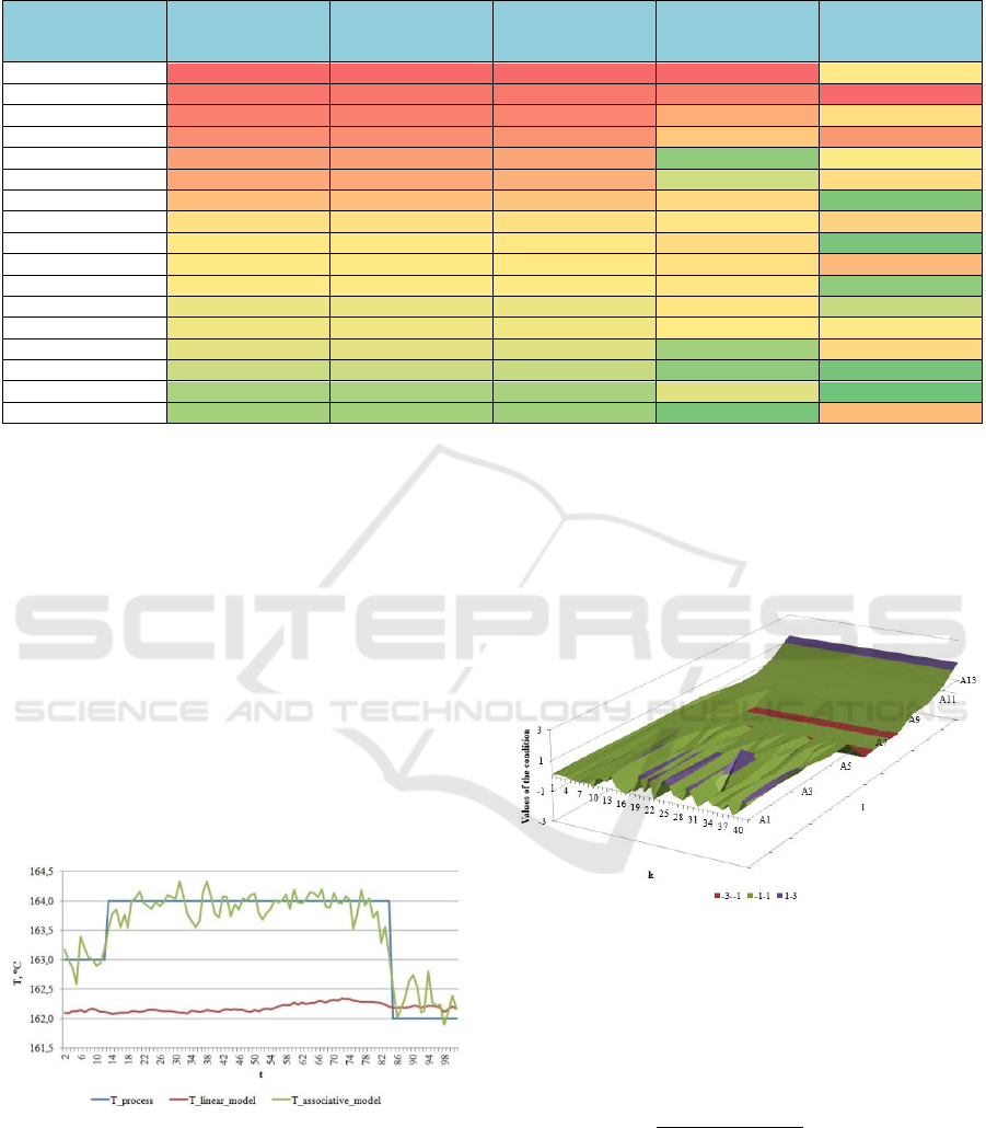
Table 1: The comparison of the associative models quantity in accordance to the number of vectors selected from the plant
knowledge base.
Number of vectors
in the associative
model
MAPE MAE MSE
Maximal absolute
error
Minimal absolute
error
195 0,30886% 0,50004 0,42292 3,32514 0,00011
170 0,30058% 0,48662 0,40238 3,17054 0,00093
152 0,29356% 0,47525 0,38331 2,84228 0,00020
133 0,28576% 0,46262 0,36426 2,65459 0,00064
113 0,27167% 0,43978 0,33527 2,21305 0,00010
101 0,26629% 0,43105 0,32104 2,33122 0,00019
86 0,25112% 0,40656 0,29165 2,53347 0,00002
65 0,22790% 0,36897 0,24949 2,46776 0,00027
61 0,22249% 0,36024 0,23835 2,52234 0,00002
60 0,22230% 0,35992 0,23673 2,49180 0,00042
58 0,22063% 0,35721 0,23372 2,44692 0,00003
55 0,21527% 0,34854 0,22429 2,46557 0,00007
54 0,21637% 0,35035 0,22685 2,41414 0,00013
50 0,21267% 0,34437 0,21904 2,24581 0,00021
46 0,20609% 0,33370 0,20835 2,21200 0,00002
42 0,19653% 0,31823 0,19297 2,35652 0,00001
41 0,19486% 0,31556 0,18879 2,17517 0,00041
on the basis knowledge about the plant, which is
updated and specified in the time progress. To
determine a necessary quantity of input vectors to
build an accurate associative model, by use of a test
sample (2400 steps) we will use a number of accuracy
and prediction adequacy evaluations. Table 1
contains 17 variants of the number of input vectors,
on the basis of which the associative models were
being built, for which indicators of the model
accuracy have been calculated: MAPE, MAE, MSE,
maximal and minimal absolute errors. From the
considered models the best associative model has
been selected, i.e. most accurate and with smallest
quantity of large errors, namely, the one built on the
basis of 42 vectors selected from the plant knowledge
base.
Figure 1: Boiling away point prediction of the 10% fraction
''150-250ºC'' at steps 2-101.
The considered process prediction was being built
on the basis of the linear and associative models form
10525 steps (1 step = 10 min.). Figure 1 displays
results of modelling for steps 2,101
, where the
dependencies of data of laboratory analysis of the
boiling away temperature of the 10% fraction ''150-
250ºC'' (T_process) of the time t, the dependence of
predictions of the boiling away temperature of the
10% fraction “150-250ºC” on the basis of the linear
model (T_linear_model) an associative model
(T_associative_model) of the time t.
Figure 2: Stability condition of the approximating part for
the prediction model in the point t=55 in the dependence of
the expansion depth.
For model (42), Figure 2 display an example of
meeting the stability criterion for the approximating
part:
∑
,
1
2
,
1.
in the dependence of the expansion depth.
Wavelet Analysis based Stability Conditions of a Prediction Model
713

5 CONCLUSIONS
In the paper, the results, obtained on the basis of the
multi-scale wavelet transform, of the stability
conditions of prediction models based on the
associative search technique and proving the
prediction without accounting possible future states
of the prediction ground.
The stability conditions obtained can be applied to
the risk potential evaluation (Kalashnikov and
Sakrutina, 2018) of implementing the prediction by
use, for instance, the Harrington verbal-numerical
scale (Harrington, 1965).
REFERENCES
Bakhtadze, N.N., Pavlov, B.V., Sakrutina, E.A., 2013.
Development of Intelligent Identification Models and
Their Applications to Predict the Submarine Dynamics
by Use of Computer Simulation Complexes. In IFAC-
PapersOnLine, vol. 7, no. 1. pp. 1244-1249.
Bakhtadze, N.N., Sakrutina, E.A., 2015. The Intelligent
Identification Technique with Associative Search. In
International Journal of Mathematical Models and
Methods in Applied Sciences, vol. 9, pp. 418-431.
Breidenstein, B., Mörke, T., Hockauf, R., Jörn Ostermann,
J., Spitschan, B., 2017. Sensors, data storage and
communication technologies. In book “Cyber-Physical
and Gentelligent Systems in Manufacturing and Life
Cycle. Genetics and Intelligence - Keys to Industry
4.0”. Academic Press, pp. 7-278.
Castello, G., Moretti, P., Vezzani, S., 2015. Retention
models for programmed gas chromatography. In
Journal of Chromatography A, vol. 1216, no. 10, pp.
1607-1623.
Ghanem, R., Romeo, F., 2000. A wavelet-based approach
for the identification of linear time-varying dynamical
systems. In Journal of Sound and Vibration, vol. 234,
no. 4, pp. 555-576.
Ghanem, R., Romeo F., 2001. A wavelet-based approach
for model and parameter identification of non-linear
systems. In International Journal of Non-Linear
Mechanics, vol. 36, no, 5, pp. 835-859.
Grossman, A., Morlet, J. 1984. Decomposition of Hardy
functions into square integrable wavelets of constant
shape. In SIAM Journal on Mathematical Analysis, vol.
14, no. 4, pp. 723-736.
Harrington, E.C., 1965. The desirable function. In
Industrial Quality Control, vol. 21, no. 10, pp. 494-498.
Kalashnikov, A., Sakrutina, E., 2018. Towards Risk
Potential of Significant Plants of Critical Information
Infrastructure In Proceedings of 2018 International
Russian Automation Conference (RusAutoCon), IEEE
Catalog Number CFP18RUS-ART, pp. 1-6.
Kassam, S., 1977. The mean-absolute-error criterion for
quantization. In Acoustics, Speech, and Signal
Processing, 1977 IEEE International Conference on
Acoustics (ICASSP '77), vol. 2, pp. 632-635.
Kim, K.-Y., Park, J., Sohmshetty, R. 2017. Prediction
measurement with mean acceptable error for proper
inconsistency in noisy weldability prediction data. In
Robotics and Computer-Integrated Manufacturing, vol.
43, pp. 18-29.
Kwakernakk, H., Sivan, R., 1972. Linear optimal control
systems. Wiley-interscience, NewYork.
Mallat, S., 1999. A wavelet tour of signal processing,
Academic press, Amsterdam.
Muto, A., Anandakrishnan, S., Alley, R.B., Horgan, H.J.,
Parizek, B.R., Koellner, S., Christianson, K., Holschuh,
N., 2019. Relating bed character and subglacial
morphology using seismic data from Thwaites Glacier,
West Antarctica. In Earth and Planetary Science
Letters, vol. 507, pp. 199-206.
Sakrutina, E., Bakhtadze, N., 2015. Towards the Possibility
of Applying the Wavelet Analysis to Derive Predicting
Models. In IFAC-PapersOnLine,
vol. 48, no. 1, pp.
409-414.
Toledo, E., Gurevitz, O., Hod, H., Eldar, M., Akselrod, S.
1998. The use of a wavelet transform for the analysis of
nonstationary heart rate variability signal during
thrombolytic therapy as a marker of reperfusion. In
Computers in Cardiology, vol. 25, pp. 609-612.
Tsatsanis, M., Giannakis, G., 2002. Time-varying system
identification and model validation using wavelets. In
IEEE Transactions on Signal Processing, vol. 41, no.
12, pp. 3512-3523.
Wei, H.L., Billings, S.A., 2002. Identification of time-
varying systems using multiresolution wavelet models.
In International Journal of Systems Science, vol. 33, no.
15, pp. 1217-1228.
Wen, X., Zhou, X., 2009. Research and Design of
Intelligent Wireless Harmonic Detection of Electric
Power System. In Proceedings of 2009 First
International Workshop on Education Technology and
Computer Science, vol. 1, pp. 644-648.
Wen, F., Zhou, Z., Qiao, J., 2010. Notice of Retraction Use
Matlab to Realize Acceleration Signal Processing of
Armor-Piercing Bullet Penetrating Steel Target. In
Proceedings of 2010 2nd International Conference on
Information Engineering and Computer Science, pp. 1-
4.
Xiao-qing Yuan, Yi-kai Shi, 2008. Characteristic spectrum
research in ae signals based on wavelet analysis. In
Proceedings of 2008 Symposium on Piezoelectricity,
Acoustic Waves, and Device Applications, pp. 439- 442.
ICINCO 2019 - 16th International Conference on Informatics in Control, Automation and Robotics
714
