Hybrid DDPG Approach for Vehicle Motion Planning
´
Arp
´
ad Feh
´
er
1 a
, Szil
´
ard Aradi
1 b
, Ferenc Heged
˝
us
1 c
, Tam
´
as B
´
ecsi
1 d
and P
´
eter G
´
asp
´
ar
2 e
1
Department of Control for Transportation and Vehicle Systems,
Budapest University of Technology and Economics, Budapest, Hungary
2
Computer and Automation Research Institute, Hungarian Academy of Sciences, Budapest, Hungary
Keywords:
Reinforcement Learning, Motion Planning, Autonomous Vehicles, Automotive Control.
Abstract:
The paper presents a motion planning solution which combines classic control techniques with machine learn-
ing. For this task, a reinforcement learning environment has been created, where the quality of the fulfilment
of the designed path by a classic control loop provides the reward function. System dynamics is described by
a nonlinear planar single track vehicle model with dynamic wheel mode model. The goodness of the planned
trajectory is evaluated by driving the vehicle along the track. The paper shows that this encapsulated problem
and environment provides a one-step reinforcement learning task with continuous actions that can be handled
with Deep Deterministic Policy Gradient learning agent. The solution of the problem provides a real-time
neural network-based motion planner along with a tracking algorithm, and since the trained network provides
a preliminary estimate on the expected reward of the current state-action pair, the system acts as a trajectory
feasibility estimator as well.
1 INTRODUCTION AND
MOTIVATION
Highly automated and autonomous driving is ex-
pected to enhance the quality of road transportation
in multiple aspects, such as increasing the level of
safety while reducing fuel consumption and emis-
sions. The development potential makes the topic one
of the most intense research fields both for vehicle in-
dustry and related academic institutions. This paper
deals with the problem of feasible motion planning,
i.e. the design and evaluation of the trajectory that the
vehicle must follow.
Many different approaches have been evolved
over the years to solve the motion planning prob-
lem for wheeled vehicles, all having advantages and
drawbacks as well. Geometric approaches assem-
ble the path of the vehicle from geometric curves as
clothoids, circular arcs and splines. A popular choice
is to define curvature as function of arc length (Li
et al., 2015). They are often used in simple low-
a
https://orcid.org/0000-0002-9491-4211
b
https://orcid.org/0000-0001-6811-2584
c
https://orcid.org/0000-0002-8063-6054
d
https://orcid.org/0000-0002-1487-9672
e
https://orcid.org/0000-0003-3388-1724
dynamic scenarios e.g. automatic parking (Vorobieva
et al., 2013). While these algorithms are computa-
tionally cheap, the ability to consider the nonholo-
nomic dynamics of the vehicle is limited to the usage
of maximal steering angle and geometric acceleration
constraints (Minh and Pumwa, 2014). Other popu-
lar methods used for trajectory planning are based
on graph search techniques. The configuration space
(space of possible states) of the vehicle is discretized
or sampled in a random manner to build a graph
of safely reachable and unoccupied states (Palmieri
et al., 2016). The shortest connection defined by
a suitably chosen metric is then searched along the
graph via some heuristics (Gammell et al., 2015). The
formulation of graph search based methods makes it
easy to deal with collision avoidance, but vehicle dy-
namics considerations are again hard to incorporate.
Variational methods are formulating the motion plan-
ning as a nonlinear optimization problem which en-
ables the usage of almost arbitrary vehicle models
(Singh et al., 2017). These methods are proven to be
able to generate dynamically feasible trajectories even
in case of high-dynamic scenarios, but this comes at
a price of high computational requirements which of-
ten make real-time applications impossible (Heged
¨
us
et al., 2017a).
Besides the classical methods, approaches based
422
Fehér, Á., Aradi, S., Heged˝us, F., Bécsi, T. and Gáspár, P.
Hybrid DDPG Approach for Vehicle Motion Planning.
DOI: 10.5220/0007955504220429
In Proceedings of the 16th International Conference on Informatics in Control, Automation and Robotics (ICINCO 2019), pages 422-429
ISBN: 978-989-758-380-3
Copyright
c
 2019 by SCITEPRESS – Science and Technology Publications, Lda. All rights reserved

on artificial neural networks gain more and more in-
terest thanks to their high performance in learning,
adaptation and generalization. Supervised learning
techniques were used for motion prediction of road
vehicles (Yim and Oh, 2004) as well as motor control
for industrial robots in dynamic environments (Liu
et al., 2017). In recent years, reinforcement learn-
ing (RL) was also used successfully for motion plan-
ning of car-like mobile robots. In (Tai et al., 2017)
authors offer a method for path planning of a mo-
bile robot to reach a specified target position without
having a-priori map information, while (Chen et al.,
2017) deals with motion planning in pedestrian-rich
environments. In (Li et al., 2019) continuous lateral
control for racetrack simulation is taught, in (Paxton
et al., 2017) the authors combine the MTCS method
with RL techniques for simple maneuvers.
The main drawback of classical optimization
based techniques despite their outstanding perfor-
mance is the necessity of computationally intensive
on-line optimization considering complex vehicle dy-
namics. With the application of reinforcement learn-
ing it is however possible to teach an artificial neu-
ral network how to drive a vehicle model with same
level complexity in an optimal way. With this ap-
proach the computationally demanding tasks can be
carried out off-line (Plessen, 2019). The motivation of
the paper is to create a trajectory planning and track-
ing algorithm especially for road vehicles that can
provide dynamically feasible motions under real-time
constraints.
The DDPG planner presented trains itself for the
optimal trajectory planning problem with predefined
initial and end states as described in Section 3.1 ,
without considering any obstacles, though regard to
dynamics described in Section 3.2. The output of the
system is a detailed trajectory curve which can be fol-
lowed by a lateral controller. The evaluation of the
resulted control loop considers angle and distance er-
rors, and side slip as a measure of feasibility.
2 PLANNER DESIGN WITH DEEP
REINFORCEMENT LEARNING
2.1 Reinforcement Learning
In problems like the one discussed in this paper, the
training of the Artificial Neural Network (ANN) lacks
training data, hence the machine learning process
needs to generate its own experiences through trial-
and-error forming a reinforcement learning frame-
work. In this area, the learner and decision maker
algorithm is called the agent. Everything outside the
agent is called the environment. The environment
shall provide the following information to the agent:
• state (output)
• action (input)
• reward (output)
The learning process consists of episodes, which is a
solution attempt for the original problem with a given
set of initial parameters, and generally an episode
consists of a series of steps. The agent interacts with
the environment, and based on the state information
provided, it selects actions, resulting in a new state
representing the new situation in every step. Further-
more, the environment provides information about
how well the agent does its job as a scalar value,
called the reward.
An overview of the developed trajectory designer
can be seen in Fig. 1: In each episode, the agent re-
ceives the initial conditions and the target for trajec-
tory planning and calculates the interior points of the
trajectory, then we drive a vehicle along the planned
route (control loop), while its performance is evalu-
ated. The reward value after the evaluation is received
by the learning agent. Thereafter the process starts
from the beginning. This is a one-step return learn-
Figure 1: Agent-environment interaction in reinforcement
learning.
ing task, meaning that an episode consists of one step
and does not considers the next state (gray in Fig. 1)
which reduces the complexity of the learning.
2.2 Deep Deterministic Policy Gradient
Method
In our previous studies, we trained reinforced learning
agents in vehicular tasks (B
´
ecsi et al., 2018)(Feh
´
er
et al., 2018)(Aradi et al., 2018) where the agents
control the environment through discreet actions, but
most vehicle control tasks and the motion planning
environment must be controlled by continuous ac-
tions. We have chosen a relatively easy-to-implement
but well-performing learning agent for this continu-
ous approach, called Deep Deterministic Policy Gra-
dient (DDPG). It is a model-free, off-policy actor-
critic algorithm using deep function approximators
that can learn policies in high-dimensional, continu-
ous action spaces (Lillicrap et al., 2015). It is based
Hybrid DDPG Approach for Vehicle Motion Planning
423

on the deterministic policy gradient (DPG) algorithm
(Silver et al., 2014). The actor µ(s|θ
µ
) specifies the
current policy by deterministically mapping states to
a specific action and the critic Q(s, a) use the Bellman
equation. The actor is updated by the a following rule:
∇
θµ
J ≈ E
S
t
∼ρ
β
[∇
θµ
Q(s,a|θ
Q
)|
s=s
t
,a=µ(St|θ
µ
)
] (1)
3 TRAINING ENVIRONMENT
As it was previously mentioned, the agent needs an
environment where it can act and learn. Such environ-
ment must consist at least the following subsystems:
• Feasible conditions based trajectory generator
module
• Nonlinear planar single track vehicle model with
dynamic wheel model
• Longitudinal and lateral control
• Reward calculation
3.1 Trajectory Generation
The trajectory planning task works with the inputs of:
the vehicle state at the start and also the desired end
state. Based on these information, the learning agent
determines the intermediate points of the trajectory.
We give an example case for the training, where
the initial state vector (2) of position and yaw angle
are fixed to the position of the vehicle, and a constant
speed of (90km/h) is chosen as a typical speed for
main roads . The final state (3) is evenly distributed
random vector drawn from a set of states, that are bit
wider than the feasible targets (3). Too many sam-
ple from unfeasible target end-states could lengthen
the learning process and hence need to be avoided,
though some is beneficial to learn the boundaries.

x
s
y
s
ψ
s
v
s

T
=

0 0 0 25m/s

T
(2)



x
e
y
e
ψ
e
v
e



=



3 ∗ v
start
rand(−y
max
,y
max
)
0.1 ∗ ψ
max
+ rand(0,1) ∗ 1.3 ∗ ψ
max
v
start



(3)
R
min
= 0.1207 ∗v
start
2.4736
(4)
y
max
= R
min
−
q
R
min
2
− x
e
2
(5)
ψ
max
= −2 ∗arctan(y
e
/x
e
)) (6)
The planned trajectory is validated by a dynamic vehi-
cle model. The feasible final state can be determined
by an empirical formula (4) as a rule of a thumb,
which gives the smallest arc radius that an average
vehicle can take at fix speed under normal conditions.
Determining the initial and the end state , the
learning agent determines y coordinate of two inter-
mediate points, placed equally between the initial and
the end points along the x coordinate. A spline is in-
serted based on the four holding points, taking into
account the initial and end gradients, which gives the
desired trajectory.
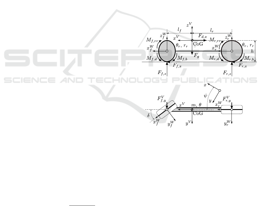
3.2 Vehicle Model
In order to provide an accurate prediction of the ve-
hicle’s behavior at fair computational requirements,
a nonlinear planar single track vehicle model con-
taining a dynamic wheel model as well is applied.
This model can deliver feasible results even in case
of high-dynamic driving maneuvers, but is simple
enough to keep its run time at a suitable level
(Heged
¨
us et al., 2017b).
Figure 2: Nonlinear single track vehicle model.
The multi-body model (Fig. 2) consists of the ve-
hicle chassis and two virtual wheels connected rigidly
representing the front and rear axles. The main pa-
rameters are the mass m and moment of inertia θ of
the chassis, the horizontal distances between the ve-
hicle’s center of gravity and the front and rear wheel
centers l
f
and l
r
, the center of gravity height of the
vehicle h, the moments of inertia θ
[ f /r]
as well as the
radii r
[ f /r]
of the front and rear wheels. The param-
eters of the wheel models have also a vital influence,
the most important ones are the coefficient of friction
µ
[ f /r]
and the parameters of the Magic Formula slip
curves C
[ f /r],[x/y]
, B
[ f /r],[x/y]
, E
[ f /r],[x/y]
which influ-
ence the transmittable amount of force between road
and tires (Pacejka, 2012).
ICINCO 2019 - 16th International Conference on Informatics in Control, Automation and Robotics
424

The inputs of the model are the steering angle of
front wheel δ (the rear wheel is considered unsteered)
and the total driving M
d
and braking M
b
torques ap-
plied at the wheels (no powertrain is modelled). The
driving torque is distributed to the front and rear axles
M
[ f /r],d
by time-varying distribution factor ξ
M
. For
the braking torque, ideal distribution M
[ f /r],b
is con-
sidered which maintains equal brake slips.
The chassis can move longitudinally x and later-
ally y and rotate ψ about its vertical axis (yaw move-
ment). The wheels can only rotate φ
[ f /r]
about their
own horizontal axes, and their longitudinal and lateral
slips s
[ f /r],[x/y]
are modelled dynamically. In the fol-
lowing superscripts are used to distinguish dynamic
quantities in ground-fixed (no superscript), vehicle-
fixed (V ) and wheel-fixed (W ) coordinate systems and
dot notation (˙) is used for time derivatives.
The dynamic equations for the chassis are derived
in the ground-fixed inertial coordinate system using
Newton’s second law for translation and rotation as
follows:
¨x =
1
m
(F
f ,x
+ F
r,x
+ F
d,x
), (7)
¨y =
1
m
(F
f ,y
+ F
r,y
+ F
d,y
), (8)
¨
ψ =
1
θ
(l
f
F
V
f ,y
− l
r
F
V
r,y
), (9)
where F
[ f /r],[x/y]
are tire forces. The aerodynamic drag
forces are calculated as:
F
V
d,x
=
1
2
c
D
A
f
ρ
A
˙x
V
p
˙x
V
+ ˙y
V
, (10)
F
V
d,y
=
1
2
c
D
A
f
ρ
A
˙y
V
p
˙x
V
+ ˙y
V
, (11)
where c
D
is the drag coefficient and A
f
is the frontal
area of the vehicle, and ρ
A
is the mass density of air.
The tire forces can be derived considering the mo-
tion of the wheels. The front and rear wheels are
modelled equally, so only the equations for the front
one are presented. The dynamic equations of the front
wheel using Newton’s second law for rotation and dy-
namic slip equations from (Pacejka, 2012) are the fol-
lowing:
¨
φ
f
=
1
θ
f

M
f ,d
− r
f
F
W
f ,x
− M
f ,b
− M
f ,rr

, (12)
˙s
f ,x
=
1
l
f ,x

r
f
˙
φ
f
− ˙x
W
f
− |˙x
W
f
|s
f ,x

, (13)
˙s
f ,y
=
1
l
f ,y

− ˙y
W
f
− |˙x
W
f
|s
f ,y

, (14)
where ˙x
W
f
and ˙y
W
f
are the longitudinal and lateral ve-
locities of wheel center. The longitudinal and lateral
slip dependent relaxation lengths are:
l
f ,[x/y]
=max

l
f ,[x/y],0

1 −
B
f ,[x/y]
C
f ,[x/y]
3
|s
f ,[x/y]
|

,
l
f ,[x/y],min

,
(15)
where l
f ,[x/y],0
is the values at standstill and l
f ,[x/y],min
are the values at at wheel spin or wheel lock. The
rolling resistance torque M
f ,rr
is calculated according
to standard SAE J2452. The longitudinal and lateral
tire forces are calculated by the Magic Formula:
˜
F
W
f ,[x/y]
=µ
f
F
W
f ,z
sin{C
f ,[x/y]
arctan(B
f ,[x/y]
˜s
f ,[x/y]
−
E[B
f ,[x/y]
˜s
f ,[x/y]
− arctan(B
f ,[x/y]
˜s
f ,[x/y]
)])}.
(16)
For the force calculation, damped slip values are used
to improve the stability of numerical solution:
˜s
f ,x
= s
f
x
+
k
f ,x
B
f ,x
C
f ,x
µ
f
F
W
f ,z
(r
f
˙
ρ
f
− ˙x
W
f
), (17)
˜s
f ,y
= s
f ,y
, (18)
where k
f ,x
is the velocity dependent damping factor
calculated as:
k
f ,x
=



1
2
k
f ,x,0

1+cos

π
| ˙x
W
f
|
v
low

,if ˙x
W
f
≤v
low
0,if ˙x
W
f
> v
low
,
(19)
with k
f ,x,0
being the damping value at zero veloc-
ity and v
low
being the velocity at which damping is
switched off. The superposition of longitudinal and
lateral forces is considered using the fiction ellipse
method:
F
W
f ,x
= sign(˜s
f ,x
)
v
u
u
t
(
˜
F
W
f ,x
˜
F
W
f ,y
)
2
(
˜
F
W
f ,y
)
2
+ (
˜s
f ,y
˜s
f ,x
˜
F
W
f ,x
)
2
F
W
f ,y
= sign(˜s
f ,y
)
v
u
u
t
(
˜
F
W
f ,x
˜
F
W
f ,y
)
2
(
˜
F
W
f ,x
)
2
+ (
˜s
f ,x
˜s
f ,y
˜
F
W
f ,y
)
2
(20)
The presented wheel model enables the usage of
explicit ODE (Ordinary Differential Equation) solvers
(e.g. the 4
th
order Runge-Kutta method) with a mod-
erate step size of approximately 1 ms. The model was
originally implemented in Python, but even with this
time step the run time was infeasible considering the
large amount of iterations in the learning process. Be-
cause of this, the vehicle model as well as the solver
was implemented in C which resulted in a tenfold in-
crease in speed approximately.
Hybrid DDPG Approach for Vehicle Motion Planning
425

3.3 Longitudinal and Lateral Control
For driving along the vehicle on the trajectory we de-
veloped a longitudinal and lateral control. The begin-
ning of the episode, the vehicle does not start with
0 km/h, therefore in order to get stabilized states the
vehicle modeluses a warm up distance to reach the
initial state. For longitudinal control tasks a simple
PID can effectively handle the problem. The Stan-
ley method (Thrun et al., 1970) is used for the lateral
control.
δ = −

ψ + arctan

k ∗
y
v

(21)
where ψ is the yaw error at the front axle, y is the
lateral error at the front axle, v is the vehicle speed
(computed at the front axle, it’s direction is parallel to
the front wheel) and k is the gain factor.
At the output of the Stanley controller, speed-
sensitive saturation was applied.
3.4 Reward Calculation
In each training step, the agent receives the state vec-
tor (initial conditions of the trajectory) and determines
its actions, the intermediate points. To calculate the
reward, the vehicle goes along the trajectory using
the internal lateral and longitudinal controls. Each
episode of the training process lasts as long as the ve-
hicle does not reach the end of the trajectory unless a
terminating condition stops it.
Defining the reward function for the agent, the
following requirements were considered, from which
terminating conditions are:
• The lateral distance error is more than 10 meters
• The longitudinal or lateral slip is higher than 0.1
• The maximum number of steps is more than 2500
• The (Yaw) angle error is more than 0.2 radians
Besides terminating conditions the sum slip and the
angular and distance deviation requirements describe
the quality features of the performance of the agent.
The episode reward consists of three weighted com-
ponents.
R
episode
= s
w
∗ R
slip
+ d
w
∗ R
dist
+ a
w
∗ R
angle
(22)
The environment defines 10 checkpoints (cp) equally
distributed on the trajectory. The distance (R
dist
)
and the angle (R
angle
) rewards were calculated at the
checkpoints and the slip reward (R
slip
) was calculated
at all time step. The subreward values are defined to
be in range [0,3] and are calculated as follows:
R
slip
= 3 −
max step
∑
step=1
−abs(max(s
[ f /r],[x/y]
))/10 (23)
R
angle
= 3 −
10
∑
cp=1
−abs(ψ) ∗2 ∗ pos (24)
R
dist
= 3 −
10
∑
cp=1
−abs(y/3) ∗ 2 ∗ pos (25)
Where ψ is the yaw error at the front axle, y is the lat-
eral error and the pos the vehicle position on the tra-
jectory. The inital value and the equations are deter-
mined by experience. When a terminating condition
rises, the episode is stopped, and the agent is given
a negative reward (R ≈ −10). The environment in-
cludes a reset method to restore the vehicle to its ini-
tial position.
4 RESULTS
Reinforcement learning algorithms usually needs a lot
of iteration. The success of the training process de-
pends on many parameters. It is highly affected by
the hyperparameters of the training algorithm, and -
in the recent case - the efficiency of the longitudinal
and lateral control, the feasible conditions from the
trajectory generator module and the consistent reward
function are also influential.
In the present case, the most significant hyperpa-
rameters are the actor and the critic network learn-
ing rates (α
a
), (α
c
), the action bound factors (a
f n
),
(a
f f
) and the Ornstein-Uhlenbeck noise parameters
(µ), (σ), (θ).
The hyperparameters of the neural network kept
constant during the iterations. During the develop-
ment process, it became clear, how strongly the re-
ward function shape and parameters affect the learn-
ing and the results. After several iterations the chosen
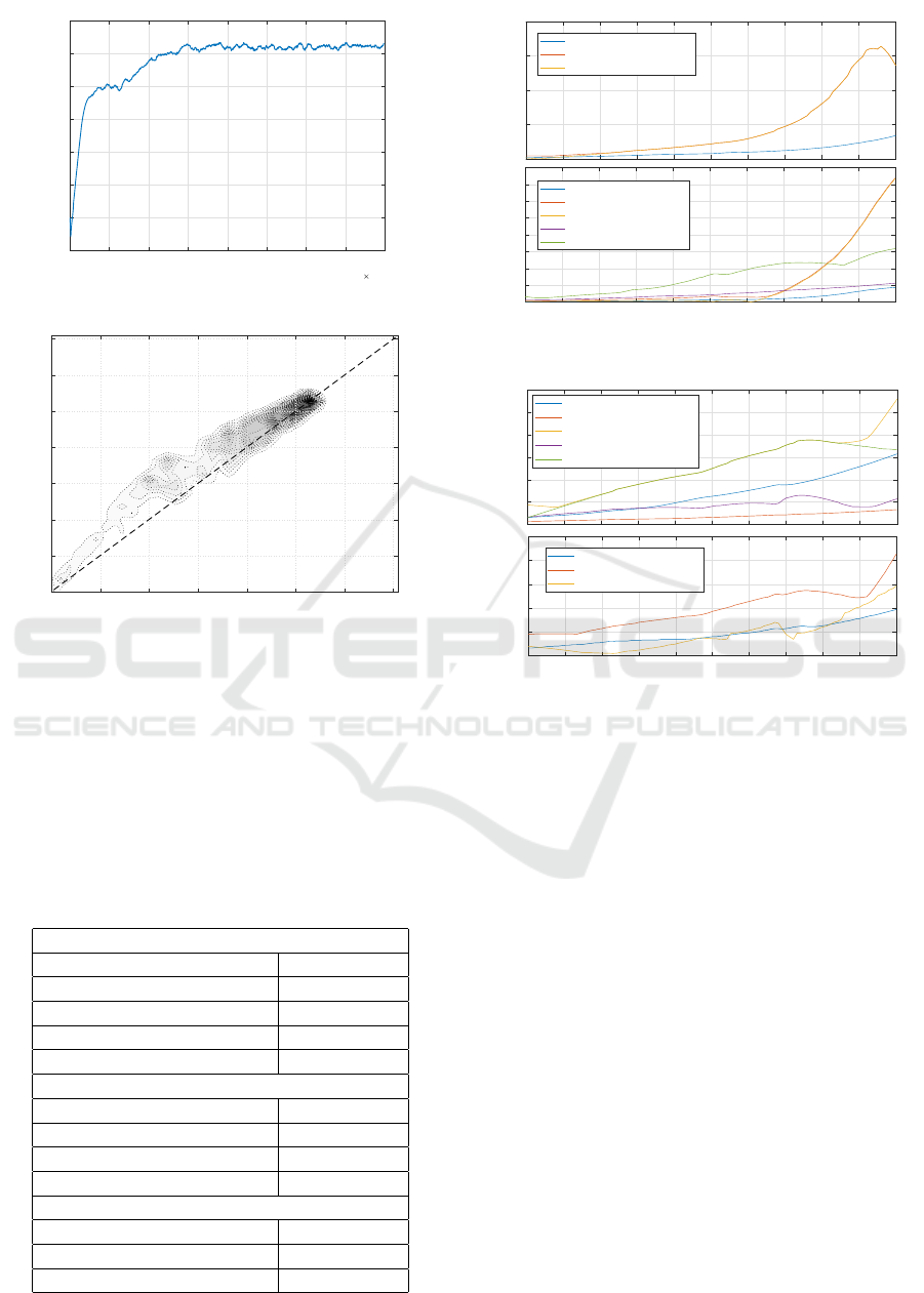
hyperparameters are summarized in Table 1. The fol-
lowing figures show the result after 80000 episodes
training. After approx. 40000 the agent started to
produce trajectories of good quality. Fig. 3 shows
the trend of the max Q-value, smoothed by moving
average using window length of 21 episodes. The di-
agram shows that the max q-value are stabilized. The
critic network learned the reward function well. The
evaluation of the learning is almost perfect based on
the Density plot (Fig. 4) which shows the estimated
Q values versus the actual rewards, as sampled from
test episodes. The diagram shows strong positive cor-
relation.
ICINCO 2019 - 16th International Conference on Informatics in Control, Automation and Robotics
426

0 1 2 3 4 5 6 7 8
Episodes
10
4
-0.5
0
0.5
1
1.5
2
2.5
3
Max Q value
Figure 3: Training Q-values.
0.5 1 1.5 2 2.5 3
Reward
0.5
1
1.5
2
2.5
3
Max Q value
Figure 4: Density plot.
For the performance evaluation of the learned
agent we differentiate two type of situations repre-
sented by different trajectory types. The first one (Fig.
6) is when the vehicle needs to turn the second one
(Fig. 5) which is the avoiding situation. In the first
case, the target angle is a higher value, however in
case of the second, it is close to zero. The target angle
of the turning maneuver depends on the distance.
Table 1: Hyperparameters.
Actor network
Learning rate (α) 0.0001
Batch size 64
Hidden F.C. layer structure [128,100,64]
Activation function relu
Output scale factor [2,4]
Critic network
Learning rate (α) 0.001
Discount factor (γ) 0.99
Hidden F.C. layer structure [128,64]
Activation function relu
Ornstein-Uhlenbeck parameters
(µ) [0,0]
(σ) 0.3
(θ) 0.15
0
0.5
1
1.5
2
Distance error avg. [m]
Max distance error [m]
Distance error at the end [m]
0 1 2 3 4 5 6 7 8 9 10
Target y [m]
0
0.05
0.1
0.15
0.2
0.25
0.3
0.35
Angle error avg. [rad]
Max. angle error [rad]
Angle error at the end [rad]
Sum. slip avg.
Max slip
Figure 5: Avoidance maneuver performance.
0
0.05
0.1
0.15
0.2
0.25
0.3
Distance error avg. [m]
Sum. slip avg.
Max distance error [m]
Max slip
Distance error at the end [m]
0 1 2 3 4 5 6 7 8 9 10
Target y [m]
0
0.005
0.01
0.015
0.02
Angle error avg. [rad]
Max. angle error [rad]
Angle error at the end [rad]
Figure 6: Turning maneuver performance.
Considering the previously defined maximum
speed the evaluation of these cases were carried out
at vehicle speed of 90km/h with a test set that is
slightly broader than the area which was considered
theoretically feasible beforehand. The diagrams show
that the planner solves these situations well. The di-
agrams also show that, the harder the situation gets,
the error of the realization also increases. Especially
at the case of the avoidance maneuver the theoretical
bounds tend to be valid (see Fig. 5). Additionally
the critic network gives a previous estimate about the
physical feasibility of planned trajectory besides the
learned optimal trajectory planner (actor network). It
can have pragmatic meaning in terms of a decision
model of control system of autonomous vehicles.
5 CONCLUSIONS
The paper presents a possible motion planner ap-
proach, with the application of Deep Deterministic
Policy Gradient based reinforcement learning com-
bined with classic control solutions. The results
Hybrid DDPG Approach for Vehicle Motion Planning
427

showed that the combination of AI and classic ap-
proach can make a good tool for designing effective
solutions for autonomous vehicle control, where addi-
tional information on the feasibility and stability can
be acquired.
The algorithm shows convergence during the
learning hence, the trained agent is basically capable
to generate effective trajectories. The visual inspec-
tion of the situations shows that the overall behavior
of the agent fulfills the requirements.
Further research will focus on extending the envi-
ronment with a variable speed solution and real-world
tests.
ACKNOWLEDGEMENTS
The research reported in this paper was supported by
the Higher Education Excellence Program of the Min-
istry of Human Capacities in the frame of Artificial
Intelligence research area of Budapest University of
Technology and Economics (BME FIKPMI/FM).
EFOP-3.6.3-VEKOP-16-2017-00001: Tal-
ent management in autonomous vehicle control
technologies- The Project is supported by the Hun-
garian Government and co-financed by the European
Social Fund. Supported by The UNKP-18-3 New
National Excellence Program of The Ministry of
Human Capacities
REFERENCES
Aradi, S., Becsi, T., and Gaspar, P. (2018). Policy gra-
dient based reinforcement learning approach for au-
tonomous highway driving. In 2018 IEEE Conference
on Control Technology and Applications (CCTA),
pages 670–675. IEEE.
B
´
ecsi, T., Aradi, S., Feh
´
er,
´
A., Szalay, J., and G
´
asp
´
ar, P.
(2018). Highway environment model for reinforce-
ment learning. IFAC-PapersOnLine, 51(22):429–434.
Chen, Y. F., Everett, M., Liu, M., and How, J. P. (2017). So-
cially aware motion planning with deep reinforcement
learning. In 2017 IEEE/RSJ International Confer-
ence on Intelligent Robots and Systems (IROS), pages
1343–1350. IEEE.
Feh
´
er,
´
A., Aradi, S., and B
´
ecsi, T. (2018). Q-learning based
reinforcement learning approach for lane keeping. In
2018 IEEE 18th International Symposium on Compu-
tational Intelligence and Informatics (CINTI). IEEE.
Gammell, J. D., Srinivasa, S. S., and Barfoot, T. D. (2015).
Batch informed trees (bit*): Sampling-based optimal
planning via the heuristically guided search of im-
plicit random geometric graphs. In 2015 IEEE In-
ternational Conference on Robotics and Automation
(ICRA), pages 3067–3074. IEEE.
Heged
¨
us, F., B
´
ecsi, T., and Aradi, S. (2017a). Dynamically
feasible trajectory planning for road vehicles in terms
of sensitivity and robustness. Transportation Research
Procedia, 27:799 – 807. 20th EURO Working Group
on Transportation Meeting, EWGT 2017, 4-6 Septem-
ber 2017, Budapest, Hungary.
Heged
¨
us, F., B
´
ecsi, T., Aradi, S., and G
´
ap
´
ar, P. (2017b).
Model based trajectory planning for highly automated
road vehicles. IFAC-PapersOnLine, 50(1):6958 –
6964. 20th IFAC World Congress.
Li, D., Zhao, D., Zhang, Q., and Chen, Y. (2019). Re-
inforcement learning and deep learning based lat-
eral control for autonomous driving [application
notes]. IEEE Computational Intelligence Magazine,
14(2):83–98.
Li, X., Sun, Z., He, Z., Zhu, Q., and Liu, D. (2015). A prac-
tical trajectory planning framework for autonomous
ground vehicles driving in urban environments. In
2015 IEEE Intelligent Vehicles Symposium (IV), pages
1160–1166.
Lillicrap, T. P., Hunt, J. J., Pritzel, A., Heess, N., Erez, T.,
Tassa, Y., Silver, D., and Wierstra, D. (2015). Contin-
uous control with deep reinforcement learning. arXiv
preprint arXiv:1509.02971.
Liu, L., Hu, J., Wang, Y., and Xie, Z. (2017). Neu-
ral network-based high-accuracy motion control of a
class of torque-controlled motor servo systems with
input saturation. Strojniski Vestnik-Journal of Me-
chanical Engineering, 63(9):519–529.
Minh, V. T. and Pumwa, J. (2014). Feasible path planning
for autonomous vehicles. Mathematical Problems in
Engineering, 2014.
Pacejka, H. B. (2012). Chapter 8 - applications of tran-
sient tire models. In Pacejka, H. B., editor, Tire and
Vehicle Dynamics (Third Edition), pages 355 – 401.
Butterworth-Heinemann, Oxford, 3rd edition edition.
Palmieri, L., Koenig, S., and Arras, K. O. (2016). Rrt-based
nonholonomic motion planning using any-angle path
biasing. In 2016 IEEE International Conference on
Robotics and Automation (ICRA), pages 2775–2781.
IEEE.
Paxton, C., Raman, V., Hager, G. D., and Kobilarov, M.
(2017). Combining neural networks and tree search
for task and motion planning in challenging envi-
ronments. In 2017 IEEE/RSJ International Confer-
ence on Intelligent Robots and Systems (IROS), pages
6059–6066. IEEE.
Plessen, M. G. (2019). Automating vehicles by deep re-
inforcement learning using task separation with hill
climbing. In Future of Information and Communica-
tion Conference, pages 188–210. Springer.
Silver, D., Lever, G., Heess, N., Degris, T., Wierstra, D., and
Riedmiller, M. (2014). Deterministic policy gradient
algorithms. In ICML.
Singh, S., Majumdar, A., Slotine, J.-J., and Pavone, M.
(2017). Robust online motion planning via contrac-
tion theory and convex optimization. In 2017 IEEE
International Conference on Robotics and Automation
(ICRA), pages 5883–5890. IEEE.
ICINCO 2019 - 16th International Conference on Informatics in Control, Automation and Robotics
428

Tai, L., Paolo, G., and Liu, M. (2017). Virtual-to-real deep
reinforcement learning: Continuous control of mobile
robots for mapless navigation. In 2017 IEEE/RSJ In-
ternational Conference on Intelligent Robots and Sys-
tems (IROS), pages 31–36. IEEE.
Thrun, S., Montemerlo, M., Dahlkamp, H., Stavens, D.,
Aron, A., Diebel, J., Fong, P., Gale, J., Halpenny,
M., Hoffmann, G., Lau, K., Oakley, C., Palatucci, M.,
Pratt, V., Stang, P., Strohband, S., Dupont, C., Jen-
drossek, L.-E., Koelen, C., and Mahoney, P. (1970).
Stanley: the robot that won the DARPA Grand Chal-
lenge, volume 23, pages 1–43. Wiley InterScience.
Vorobieva, H., Minoiu-Enache, N., Glaser, S., and Mam-
mar, S. (2013). Geometric continuous-curvature path
planning for automatic parallel parking. In 2013 10th
IEEE International Conference on Networking, Sens-
ing and Control (ICNSC), pages 418–423.
Yim, Y. U. and Oh, S.-Y. (2004). Modeling of vehicle dy-
namics from real vehicle measurements using a neural
network with two-stage hybrid learning for accurate
long-term prediction. IEEE Transactions on Vehicu-
lar Technology, 53(4):1076–1084.
Hybrid DDPG Approach for Vehicle Motion Planning
429