
Vision-based Localization of a Wheeled Mobile Robot with a Stereo
Camera on a Pan-tilt Unit
A. Zde
ˇ
sar
a
, G. Klan
ˇ
car
b
and I.
ˇ
Skrjanc
c
University of Ljubljana, Faculty of Electrical Engineering, Tr
ˇ
za
ˇ
ska 25, 1000 Ljubljana, Slovenia
Keywords:
Mobile Robots, Robot Vision, Optimal Filtering, Estimation Algorithms, Localization, System Observability.
Abstract:
This paper is about a vision-based localization of a wheeled mobile robot (WMR) in an environment that
contains multiple artificial landmarks, which are sparsely scattered and at known locations. The WMR is
equipped with an on-board stereo camera that can detect the positions and IDs of the landmarks in the stereo
image pair. The stereo camera is mounted on a pan-tilt unit that enables rotation of the camera with respect to
the mobile robot. The paper presents an approach for calibration of the stereo camera on a pan-tilt unit based
on observation of the scene from different views. Calibrated model of the system and the noise model are then
used in the extended Kalman filter that estimates the mobile robot pose based on wheel odometry and stereo
camera measurements of the landmarks. We assume that the mobile robot drives on a flat surface. In order to
enforce this constraint, we transform the localization problem to a two-dimensional space. A short analysis
of system observability based on indistinguishable states is also given. The presented models and algorithms
were verified and validated in simulation environment.
1 INTRODUCTION
Autonomous mobile robots are one of the emerging
fields of technology that is not only expected to be-
come an inevitable part of smart factories of tomor-
row but will play an essential role in our cities and
homes of the future. Advances in the development
of intelligent and autonomous systems are paving the
way to a new breed of robotic systems that will be able
to work alongside humans in a non-intrusive, harm-
less and cooperative way. Nowadays, the self-driving
vehicles are being tested on roads in various traffic
conditions daily and some self-driving technologies
are already implemented in the most modern con-
sumer vehicles.
Autonomous mobile systems perceive the envi-
ronment through sensors. Commonly used sensors
in mobile robotics are proximity and distance sensors
(e.g. ultrasonic distance sensors, laser range scan-
ners, etc.) that enable detection of obstacles, map
building and localization. The emergence of new sen-
sor technologies and contemporary computational ca-
pabilities broaden the range of available sensors that
a
https://orcid.org/0000-0002-2254-6069
b
https://orcid.org/0000-0002-1461-3321
c
https://orcid.org/0000-0002-0502-5376
are appropriate for environment perception. Cameras
are one of the most promising sensors in the field of
mobile robotics and they are seldom used to solve
the mobile robot localization and mapping problems
(Se et al., 2001; Agrawal and Konolige, 2006; Du
and Tan, 2016; Fischer et al., 2016; Piasco et al.,
2016; Fuentes-Pacheco et al., 2015; Konolige and
Agrawal, 2008; Mei et al., 2011). The vision-based
environment mapping and localization problems are
commonly solved in the framework of Kalman filter
(Chen, 2012) or particle filter (Kim et al., 2017; Del-
laert et al., 1999).
In this paper a stereo camera is used as a sensor
for localization of a wheeled mobile robot (WMR).
The environment is sparsely scattered with artificial
landmarks at known locations that can be robustly de-
tected in each image of the stereo camera whenever
they are visible in the camera field of view. In our case
we use square-based markers that can be detected ef-
ficiently with the ArUco image processing approach
(Garrido-Jurado et al., 2016). In order to extend
the tracking range of landmarks, even when the mo-
bile robot moves around the environment, the stereo
camera is mounted on a Pan-Tilt Unit (PTU) that
enables rotation of the camera around its vertical and
544
Zdešar, A., Klan
ˇ
car, G. and Škrjanc, I.
Vision-based Localization of a Wheeled Mobile Robot with a Stereo Camera on a Pan-tilt Unit.
In Proceedings of the 16th International Conference on Informatics in Control, Automation and Robotics (ICINCO 2019), pages 544-551
ISBN: 978-989-758-380-3
Copyright
c
2019 by SCITEPRESS – Science and Technology Publications, Lda. All rights reserved

horizontal axis. This paper presents the models and
algorithm for localization of the WMR that drives on
a flat ground and observes the landmarks with a stereo
camera. This is a reasonable assumption for many
WMRs in indoor environment, and since we take this
assumption implicitly into the model a better perfor-
mance of the pose estimation can be expected. The
presented approach is therefore not suitable for legged
robots and robots that operate on uneven terrain.
The rest of the paper is structured as follows. In
Section 2 a detailed description of the system is given,
along with mathematical model of the system and cal-
ibration procedure for estimation of the parameters
that describe the static transformation of the stereo
camera on the PTU. Section 3 is about mobile robot
localization, and it presents the stochastic modelling
of the system for the purpose of localization, analysis
of the system observability and localization approach.
In Section 4 some conclusions are drawn.
2 SYSTEM DESCRIPTION
The system is shown in Fig. 1. On the WMR Pioneer
3-AT a PTU with a stereo camera is mounted. The
mobile system is also equipped with other proximity
and distance sensors, but these are not considered in
this work.
Figure 1: WMR Pioneer 3-AT with a stereo camera on a
PTU.
Let us introduce the coordinate frames that we
use: world frame W ; robot frame R (origin is in the
intersection of the robot vertical rotation axis and the
ground plane); base frame S, pan frame U and tilt
frame V of the PTU; left (right) camera frame C
1
(C
2
);
stereo camera frame C (between the left and right
camera frame); left (right) image frame P
1
(P
2
). The
transformations between the frames are represented
graphically in Fig. 2.
Static transformation that describes the pose of the
Mobile
robot
Stereo
camera
Pan-tilt
unit
World W
Robot R
Pan-tilt S
Pan U
Tilt V
Stereo camera C
Left camera C
1
Left image P
1
Right camera C
2
Right image P
2
R
W
R
, t
W
R
R
R
S
, t
R
S
R
S
U
= Rot
z
(ψ), t
S
U
= 0
R
U
V
= Rot
y
(θ), t
U
V
= 0
R
V
C
, t
V
C
R
C
C
1
, t
C
C
1
R
C
C
2
, t
C
C
2
P
C
1
P
1
P
C
2
P
2
Figure 2: Diagram of the static (solid arrows) and dynamic
(curly arrows) transformations between the frames.
PTU on the mobile robot is:
R
R
S
= I , t
R
S
=
0.154 0.023 0.563
T
, (1)
where I is an identity matrix.
The frames S, U and V have a common origin (in
the intersection of the pan and tilt rotation axes):
t
S
U
= t
U
V
= 0 ,
where 0 is the vector of zeros. Orientations of the
frames U and V , which are dependent on the pan and
tilt angles, ψ and θ, are given in (2) and (3).
R
S
U
= Rot
z
(ψ) =
cosψ −sinψ 0
sinψ cosψ 0
0 0 1
(2)
R
U
V
= Rot
y
(θ) =
cosθ 0 sinθ
0 1 0
−sin θ 0 cosθ
(3)
Notation Rot
a
(α) represents a rotation around the axis
a for the angle α.
In (4) the static transformations of the cameras
with respect to the tip of the PTU (tilt frame V ) are
given.
R
V
C
1
= R
V
C
2
= Rot
z
(−
π
2
)Rot
x
(−
π
2
)
t
V
C
1
=
0.002 0.032 0.057
T
t
V
C
2
=
0.002 −0.032 0.057
T
(4)
The values in (1) and (4) have been obtained using
the calibration procedure described in Section 2.1.
Vision-based Localization of a Wheeled Mobile Robot with a Stereo Camera on a Pan-tilt Unit
545

2.1 System Calibration
The intrinsic parameters (P
P
1
C
1
and P
P
2
C
2
) and the rel-
ative pose between the cameras (R
C
2
C
1
and t
C
2
C
1
) in
the stereo-camera setup can be determined using the
stereo camera calibration procedure (Bouguet, 2004).
Several images of the chessboard-like pattern from
different poses need to be captured. The pattern need
to be visible in both images. From the corresponding
points in the stereo image pairs and given the known
size of the pattern square, the stereo-camera parame-
ters can be obtained. If required, the calibration pro-
cedure can be extended in a way that lens distortions
are taken into account.
In our case we also need to determine the relative
pose of the stereo camera with respect to the tip of the
PTU, i.e. R
V
C
and t
V
C
. The relative pose of the stereo
camera with respect to the tip of the PTU could be
measured, but since the location of the camera frame
origin and also the location of the tip of the PTU are
not directly accessible, this is hard to do without an
error. Therefore we would like to estimate this pose
with an appropriate calibration procedure that is de-
scribed next.
Given a calibrated stereo camera we observe a set
of points on a static object in the environment (with
respect to the base frame of the PTU) from different
configurations (views) of the PTU. In the i-th config-
uration the pose of the tip with respect to the base of
the PTU is represented with rotation R
S
V,i
(the pan an-
gle is ψ
i
and the tilt angle is θ
i
). The triangulation
approach can be used to estimate the 3D positions (in
the stereo camera frame) p
C,i,l
, l = 1, 2, . . . , n, of the
observed n image points. Observing the same set of
points from m different views (configurations of the
PTU), the transformations R
C,0
C, j
, t
C,0
C, j
, j = 1, 2, . . . , m,
can be obtained from the set of points in views i = 0
and i = j in the following way. First the centres of the
points
¯
p
C,i
=
1
n
∑
n
k=1
p
C,i,k
are evaluated for each view
i, and each set of the points is given with respect to its
centre:
˜
p
C,i,k
= p
C,i,k
−
¯
p
C,i
, (5)
for every point k in every view i. The rigid transfor-
mation p
C,0,k
= R
C,0
C, j
p
C, j,k
+ t
C,0
C, j
can be determined
with the minimization of the least squares error cost
function J:
J =
n
∑
k=1
p
C,0,k
− R
C,0
C, j
p
C, j,k
− t
C,0
C, j
. (6)
Taking into account the centred set of points (5), the
criterion (6) can be written as:
J =
n
∑
k=1
˜
p
C,0,k
− R
C,0
C, j
˜
p
C, j,k
, (7)
since
¯
p
C,0
−R
C,0
C, j
¯
p
C, j
−t
C,0
C, j
= 0. The cost function (7)
has minimum where the trace(R
C,0
C, j
H
j
) has maximum
(Eggert et al., 1997), and H
j
is defined as:
H
j
=
n
∑
k=1
˜
p
C, j,k
˜
p
T
C,0,k
.
Rotation R
C,0
C, j
that maximizes the aforementioned
trace can be obtained from the Singular Value Decom-
position (SVD) of H
j
= U
j
S
j
V
T
j
:
R
C,0
C, j
= V
j
U
T
j
.
If the determinant detR
C,0
C, j
is −1 instead of +1, the
transformation represents a reflection rather than ro-
tation. In such a case the rotation can be determined
from R
C,0
C, j
= [v
j,1
, v
j,2
, −v
j,3
]U
T
j
, where the columns
are obtained from the matrix V
j
= [v
j,1
, v
j,2
, v
j,3
].
Once the rotation is known, the translation vector t
C,0
C, j
can be estimated from:
t
C,0
C, j
=
¯
p
C,0
− R
C,0
C, j
¯
p
C, j
.
More closed-form approaches that can be used to
solve the presented rigid-motion estimation problem
can be found in (Eggert et al., 1997).
The orientation of the PTU tip in the view j =
1, 2, . . . , m with respect to the view i = 0 is R
V,0
V, j
=
R
V,0
S
R
S
V, j
. The static orientation R
V
C
that is view in-
variant can be obtained from the set of relations ( j =
1, 2, . . . , m):
R
V,0
V, j
R
V
C
= R
V
C
R
C,0
C, j
. (8)
At least two sets of (8) are required to estimate R
V
C
,
therefore the pattern of points need to be observed
from at least three different configurations of the
PTU. The system of equations (8) can be written as:
R
V,0
V, j
⊗ R
C,0
C, j
− I
vec
R
C
V
= 0 , (9)
where operator ⊗ represents the Kronecker matrix
product and vec(X) is a vector with stacked columns
of the matrix X. Several different pairs of matrices
R
V,0
V, j
and R
C,0
C, j
can therefore be stacked together into
the linear form (9) that can be solved using the SVD
algorithm. Once the estimate of the rotation R
V
C
is
obtained, the translation vector t
V
C
can be determined
from the linear system of equations:
R
V,0
V, j
− I
t
V
C
= R
V
C
¯
p
C,0
− R
V,0
V, j
R
V
C
¯
p
C, j
. (10)
At least two systems like (10) need to be stacked to-
gether in order to solve for the translation vector t
V
C
.
With an appropriate modification, the presented
calibration procedure can also be used to determine
the static rotation R
R
S
and translation t
R
S
if the pose of
the mobile robot in the world coordinate frame can be
measured.
ICINCO 2019 - 16th International Conference on Informatics in Control, Automation and Robotics
546

3 LOCALIZATION
The problem of localization is about estimation of
the transformation between the world and robot frame
(R
W
R
and t
W
R
in Fig. 2). In our case we would like to
achieve this based on fusion of wheel odometry and
measurement of multiple landmarks at known loca-
tions with a stereo camera. If the WMR motion is
constrained to the ground plane, the pose of the robot
with respect to the world can be given with the gener-
alized coordinates q
T
(k) = [x(k) y(k) ϕ(k)]:
R
W
R
=
cosϕ(k) −sin ϕ(k) 0
sinϕ(k) cosϕ(k) 0
0 0 1
, t
W
R
=
x(k)
y(k)
0
,
where the coordinates x(k) and y(k) represent po-
sition and the coordinate φ(k) is orientation of the
robot. This is a reasonable assumption for many in-
door spaces since we assume that the mobile system
drives on a flat surface and that it does not tilt sig-
nificantly. We also assume that the poses of all the
static and also moving sensors on-board of the mobile
system are known at all times. This means that both
states of the PTU are measurable. All the static trans-
formations can be determined with the procedure pre-
sented in the previous section. In the following sub-
section the modelling of the system with uncertainties
is presented that takes into account different simpli-
fications. Since the mobile robot only moves along
the ground plane, the estimation problem is also con-
verted to a pure 2D estimation problem. In this paper
we also assume that the PTU is not moving during the
localization, i. e. the PTU is in its home position all
the time.
3.1 System Modelling
3.1.1 Wheeled Mobile Robot
The WMR has a differential drive (the wheels on each
side are driven jointly). The kinematic model of the
differential drive in the discrete form with the sam-
pling time T can be written as:
q(k + 1) = q(k) +
T v(k)cosϕ(k)
T v(k)sinϕ(k)
T ω(k)
,
where v(k) and ω(k) are the WMR linear and angular
velocity, respectively.
Wheels on each side of the mobile robot are
equipped with incremental encoders, therefore the
odometry can be implemented. Given the true relative
encoder readings between one sample time for the left
and right wheel u
T
(k) = [∆λ
L
(k) ∆λ
R
(k)], we assume
the following odometry model in the discrete form:
q(k + 1) = q(k) + g
λ
∆λ
R
(k)+w
R
(k)+∆λ
L
(k)+w
L
(k)
2
cosϕ(k)
∆λ
R
(k)+w
R
(k)+∆λ
L
(k)+w
L
(k)
2
sinϕ(k)
∆λ
R
(k)+w
R
(k)−∆λ
L
(k)−w
L
(k)
L
,
(11)
where g
λ
is the constant that converts the encoder
readings into relative distances and L is the distance
between the wheels — both parameters are normally
determined with calibration. The encoder readings
include a normally distributed white noise w(k) =
[w
L
(k) w
R
(k)] with zero mean. The covariance of
the noise w(k) is assumed to be increasing with the
magnitude of the encoder reading, which coincides
with the speed of the wheels, according to the model
(Tesli
´
c et al., 2011):
Q
w
(k) =
∆λ
2
L
(k)σ
2
w
L
0
0 ∆λ
2
R
(k)σ
2
w
R
.
3.1.2 Stereo Camera
We assume that we have a calibrated stereo camera
system in canonical configuration with the baseline
distance B and focal length of each camera f . The
origin of each camera image plane coincides with the
camera optical center and the axis x of the left im-
age frame is colinear with the axis x in the right im-
age frame. The projections of a single point in the
3-D space to the left and right camera image plane
are (x
l
, y
l
) and (x
r
, y
r
), respectively. Since the posi-
tions of landmarks are measured in each image with
a marker detection algorithm (Garrido-Jurado et al.,
2016), let us assume that the aforementioned variables
have normal distribution. They can be gathered in a
vector s:
s =
x
l
y
l
x
r
y
r
T
∈ N (
¯
s, Q
s
), (12)
where
¯
s is the expected value of the measurement vec-
tor s and Q
s
is the measurement noise covariance ma-
trix. The shape of the covariance matrix Q
s
is as-
sumed to be block diagonal, since the measurement
noises of the left and right camera are independent
of each other (shaking of the stereo camera rig is not
considered here):
Q
s
=
σ
2
x
l
σ
x
l
,y
l
0 0
σ
x
l
,y
l
σ
2
y
l
0 0
0 0 σ
2
x
r
σ
x
r
,y
r
0 0 σ
x
r
,y
r
σ
2
y
r
. (13)
In (13) the diagonal elements represent the variances
and the off-diagonal elements are the covariances.
Let us represent the position of a point in the 3D
camera frame. The origin of the stereo camera frame
Vision-based Localization of a Wheeled Mobile Robot with a Stereo Camera on a Pan-tilt Unit
547

C is in the middle of the line that connects the cam-
era focal points, z
C
-axis is perpendicular to the image
plane and it is pointing outwards to the scene, y
C
-axis
is parallel to the vertical image axis and x
C
-axis is
parallel to the horizontal image axis, pointing in the
direction that makes the camera frame right handed.
Here we introduce a special coordinate vector r for
presentation of the point in the stereo camera frame:
r
T
=
tanα tan β z
C
=
x
C
z
C
y
C
z
C
z
C
. (14)
This representation can uniquely represent only the
half-space in front of the camera (z
C
> 0) and it is
therefore suitable only for the cameras that have the
field-of-view smaller that π.
The position of the point r in the camera frame can
be determined from the projection vector (12) using
triangulation:
r
T
=
h
x
l
+x
r
2 f
y
l
+y
r
2 f
B f
x
l
−x
r
i
.
The variance of this estimate is therefore:
Q
r
=
σ
2
x
l
+σ
2
x
r
4 f
2
σ
x
l
,y
l
+σ
x
r
,y
r
4 f
2
−z
2
C
σ
2
x
l
−σ
2
x
r
2B f
2
σ
x
l
,y
l
+σ
x
r
,y
r
4 f
2
σ
2
y
l
+σ
2
y
r
4 f
2
−z
2
C
σ
x
l
,y
l
−σ
x
r
,y
r
2B f
2
−z
2
C
σ
2
x
l
−σ
2
x
r
2B f
2
−z
2
C
σ
x
l
,y
l
−σ
x
r
,y
r
2B f
2
z
4
C
σ
2
x
l
+σ
2
x
r
B
2
f
2
.
If we assume that the measurement noises of the
left and right camera have the same properties, the
following equivalence of variances and covariances
holds: σ
2
x
l
= σ
2
x
r
and σ
x
l
,y
l
= σ
x
r
,y
r
; and the covari-
ance matrix Q
r
becomes block diagonal. If we fur-
ther assume that the covariances are zero (σ
x
l
,y
l
=
σ
x
r
,y
r
= 0), the covariance matrix Q
r
becomes diag-
onal, where the diagonal elements are:
h
σ
2
tanα
σ
2
tanβ
σ
2
z
C
i
=
h
σ
2
x
l
2 f
2
σ
2
y
l
2 f
2
z
4
C
2σ
2
x
l
B
2
f
2
i
. (15)
From (14) the position of the point in the stereo
camera frame p
C
can be obtained:
p
T
C
=
x
C
y
C
z
C
=
z
C
tanα z
C
tanβ z
C
.
Under the assumption (15), the measurement covari-
ance matrix Q
C
of the vector p
C
in the stereo camera
frame is:
Q
C
=
z
2
C
σ
2
tanα
+ (tan α)
2
σ
2
z
C
tanαtanβσ
2
z
C
tanασ
2
z
C
tanαtanβσ
2
z
C
z
2
C
σ
2
tanβ
+ (tan β)
2
σ
2
z
C
tanβσ
2
z
C
tanασ
2
z
C
tanβσ
2
z
C
σ
2
z
C
.
(16)
The transformation of the point p
C
in the stereo
camera frame to the point p
R
in the mobile robot base
frame is p
R
= R
R
C
p
C
+ t
R
C
as defined in Section 2. The
covariance (16) can also be transformed to the mobile
robot base frame:
Q
R
= R
R
C
Q
C
(R
R
C
)
T
.
Since we are dealing with estimation of the mobile
robot that can only move in the ground plane, we can
make the projection of the 3D points to the ground
plane (z
R
= 0), i.e. the point in the 2D ground plane
is therefore p
G
= P
G
R
p
R
, where P
G
R
is the parallel pro-
jection matrix:
P
G
R
=
1 0 0
0 1 0
.
The covariance matrix Q
G
that is the projection of the
covariance matrix Q
R
can be given as:
Q
G
= P
G
R
Q
R
(P
G
R
)
T
. (17)
In the configuration when the stereo camera is in
its home position, in which case the camera axis z
C
is
aligned with the robot axis x
R
and the camera axis x
C
is in the opposite direction of the robot axis x
R
, the p
G
simplifies to:
p
T
G
=
h
B f
x
l
−x
r
+ x
R
C
−
B
2
x
l
+x
r
x
l
−x
r
+ y
R
C
i
, (18)
where x
R
C
and y
R
C
are the first and the second element
of the translation vector t
R
C
, respectively. The covari-
ance matrix (17) in this particular case is:
Q
G
=
σ
2
z
C
−tan ασ
2
z
C
−tan ασ
2
z
C
z
2
C
σ
2
tanα
+ (tan α)
2
σ
2
z
C
. (19)
The covariance matrix (19) is strongly dependent on
the distance to the measured point due to the fact
that σ
z
C
∝ z
2
C
. Top row in Figure 3 shows covari-
ances (19) as ellipses for different positions of the
landmarks overlayed over simulated noisy data. The
proposed noise model was verified with real measure-
ments (bottom row in Figure 3) by temporal observa-
tion of landmarks at various positions from a static
WMR.
The (18) represents the measurement of the point
in the ground plane. This measurement can also be
given in polar coordinates z
T
= [d θ]:
z
T
=
h
q
x
2
G
+ y
2
G
arctan
y
G
x
G
+ jπ
i
, j ∈ {0, 1}.
The stereo camera sensor can therefore be considered
as the sensor that measures the distance and angle to
the landmark. In our case we considered that the vi-
sion system can also determine the ID of the measured
landmark, therefore we can distinguish between dif-
ferent landmarks. Let us express the measurement of
the landmark with the system state vector q(k):
z(k) =
d(k)
θ(k)
=
"
p
(x
m
− x(k))
2
+ (y
m
− y(k))
2
arctan
y
m
−y(k)
x
m
−x(k)
− ϕ(k) + j(k)π
#
,
(20)
where x
m
and y
m
are the coordinates of the landmark
in the world frame.
ICINCO 2019 - 16th International Conference on Informatics in Control, Automation and Robotics
548
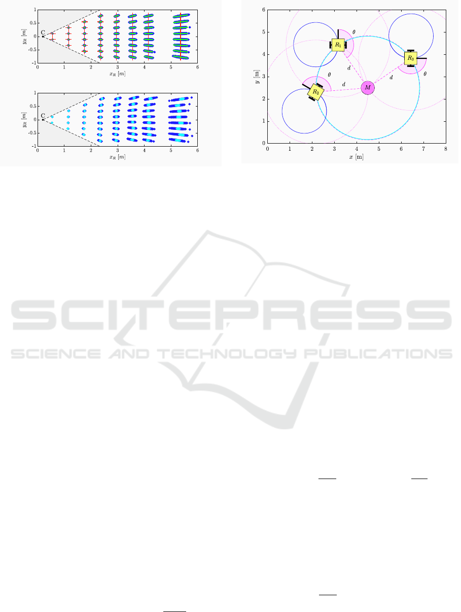
Figure 3: Top, simulation of the stereo camera measurement
noise for multiple landmarks that are in the stereo camera C
field of view (red cross – real landmark position, blue – sim-
ulated noise, green – noise covariance ellipse). Bottom, real
measurements (cyan – static camera, blue – small shaking
of the camera).
3.2 System Observability
In order to estimate system states they need to be ob-
servable. The observability of the non-linear system
can be evaluated based on the analysis of indistin-
guishable states. Briefly, two states are indistinguish-
able if for every input on a finite time interval, identi-
cal outputs are obtained. A system is observable if the
set of all the indistinguishable states of a state x con-
tains only the state x for every state x in the domain of
definition. For more detailed definition see (Hermann
and Krener, 1977).
Let us evaluate the observability of the system in
the case of only one landmark graphically. In Fig-
ure 4 we can see three robots in different poses that
all measured the same distance and angle to the land-
mark. Even if the robots move along any admissi-
ble trajectory (e.g. along the circle) there is no way
to distinguish between different robot poses based on
measured outputs. The pose of the robot q is clearly
not observable if only a single landmark is used. In a
similar way it is not hard to observe that the system is
observable if two or more landmarks are used, since
we have assumed that the IDs of the landmarks are
also known. If the later would not hold, three or more
landmarks would be required.
Now we introduce a new state vector q
T
p
(k) =
[d(k) θ(k)] that has all the states measurable directly.
The kinematic model of this system is:
q
p
(k + 1) = q
p
(k) +
"
−T v(k)cosθ(k)
T ω(k) + T v(k)
sinθ(k)
d(k)
#
. (21)
The system (21) gives only a partial information about
Figure 4: Three poses of the robots that are indistinguish-
able from the outputs in the case of a single landmark M.
the system pose (a subspace of possible robot poses),
but the system is completely observable already in the
case of a single landmark.
3.3 Extended Kalman Filter
We use Extended Kalman Filter (EKF) to solve the lo-
calization problem, which consists of a prediction and
a correction step. The pose of the mobile robot q(k)
could be estimated directly, if the model (11) would
be used in the prediction step of the EKF and the cor-
rection step would be made based on the measure-
ments (20) to all the visible landmarks.
In this paper we used a different approach, us-
ing multiple partial estimators that estimate the states
q
p,m
(k) for each visible landmark m independently.
Each partial estimator uses the model (21) in the pre-
diction step of the EKF:
ˆ
q
p,m
(k + 1) = f
p,m
(q
p,m
(k), u(k)),
ˆ
P
p,m
(k + 1) = A
p,m
(k)P
p,m
(k)A
T
p,m
(k)+
+ F
p,m
(k)Q
p,m
(k)F
T
p,m
(k) ,
where A
p,m
(k) =
∂f
p,m
∂q
p,m
k
and F
p,m
(k) =
∂f
p,m
∂w
k
. The
measurement (20) of the associated landmark is then
used in the correction of each partial estimator:
L
p,m
(k) = C
p,m
(k)
ˆ
P
p,m
(k)C
T
p,m
(k) + R
p,m
(k)
K
p,m
(k) =
ˆ
P
p,m
(k)C
T
p,m
(k)L
−1
p,m
(k)
q
p,m
(k) =
ˆ
q
p,m
(k) + K
p,m
(k)(z
p,m
(k) −
ˆ
z
p,m
(k)) ,
P
p,m
(k) =
ˆ
P
p,m
(k) − K
p,m
(k)C
p,m
(k)
ˆ
P
p,m
(k) ,
where C
p,m
(k) =
∂h
p,m
∂q
p,m
k
. The Q
p,m
(k) and R
p,m
(k)
in the EKF are defined according to the covariance
model developed in Section 3.1. In this way we do
not estimate the pose of the mobile robot, but only the
Vision-based Localization of a Wheeled Mobile Robot with a Stereo Camera on a Pan-tilt Unit
549
distances and headings of each landmark with respect
to the WMR. The estimates q
p,m
(k), m = 1, 2, . . . , M
are then merged into the estimate of the state q(k).
This can be achieved using a triangulation (or trilater-
ation) approach, e.g. using the approach presented in
(Betke and Gurvits, 1997).
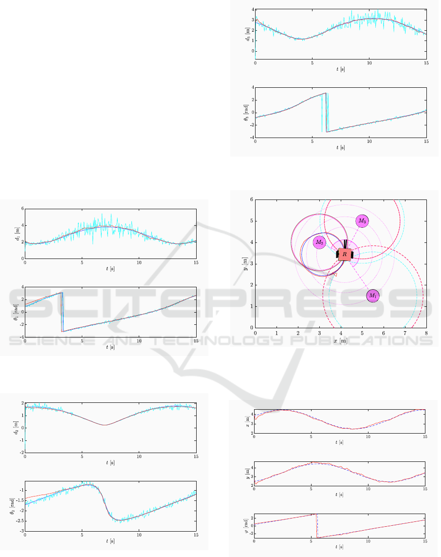
In the simulation we have used three landmarks
and the limited field of view of the camera was not
taken into account . Figures 5 to 7 present the results
of all three partial estimators. It can be seen that the
distance measurement noise is largely dependant on
the distance to the landmark, but the output of each
partial estimator converges to the true value. Based
on the outputs of these estimators, the pose of the mo-
bile robot is calculated as an intersection of all three
solutions (circles) in the least squares sense (Figure
8). The pose estimate is shown in Figure 9.
Figure 5: Estimation of the landmark 1 state vector q
p
(blue
– true, red – estimate, cyan – measurement).
Figure 6: Estimation of the landmark 2 state vector q
p
(blue
– true, red – estimate, cyan – measurement).
Figure 7: Estimation of the landmark 3 state vector q
p
(blue
– true, red – estimate, cyan – measurement).
Figure 8: Estimation of the robot pose q at the end of
time (solid blue – true pose, solid red – estimated pose,
dashed cyan – measurements, dashed red – estimated mea-
surements).
Figure 9: Estimation of the robot state vector q (blue – true,
red – estimate).
ICINCO 2019 - 16th International Conference on Informatics in Control, Automation and Robotics
550

4 CONCLUSION
Calibration of the system parameters is essential for
optimal performance of the localization algorithms.
We have showed a calibration procedure that can be
used to determine static transformation between the
camera and PTU coordinate frame. The procedure re-
quires only observation of the same set of points from
three different configurations of the PTU. This cali-
bration procedure is simple to deploy on a real set-
ting, without any special preparation of the environ-
ment solely for the calibration purposes.
In the development of the localization algorithm
system uncertainties were taken into account. Intro-
ducing the flat ground surface constraint, the consid-
ered localization problem can be solved in the two
dimensional plane where the camera measures dis-
tances and angles to the visible landmarks. Assum-
ing normally distributed noise in image measurement
of landmark points, the standard deviation increases
predominantly in the direction of the image ray, pro-
portionally to the squared distance from the camera.
We have shown an approach that uses multiple
partial Kalman filters, where each filter estimates only
the distance and heading to the particular landmark,
and the outputs of these estimators are later used to
calculate the robot pose. Results demonstrate that
this is a feasible approach that converges to the true
pose of the mobile robot. The benefit of this ap-
proach is computational efficiency, since the covari-
ance matrices are low dimensional. To reduce mem-
ory consumption during large-area localization, the
landmarks that have not been observed for a long time
can be made forgotten. The presented models are also
valid when the camera is moving. The proposed sys-
tem can be augmented with a control for tracking of
the nearest visible landmarks to reduce the time when
no landmarks are in the stereo camera field of view.
ACKNOWLEDGEMENTS
The authors acknowledge the financial support from
the Slovenian Research Agency (research core fund-
ing No. P2-0219).
REFERENCES
Agrawal, M. and Konolige, K. (2006). Real-time localiza-
tion in outdoor environments using stereo vision and
inexpensive GPS. In 18th Int. Conf. on Pattern Recog-
nition, volume 3, pages 1063–1068.
Betke, M. and Gurvits, L. (1997). Mobile robot localization
using landmarks. IEEE transactions on robotics and
automation, 13(2):251–263.
Bouguet, J.-Y. (2004). Camera calibration toolbox for Mat-
lab. [online] Available at: http://www.vision.caltech.
edu/bouguetj/calib doc [Accessed April 2019].
Chen, S. Y. (2012). Kalman filter for robot vision: a survey.
IEEE Trans. on Industrial Electronics, 59(11):4409–
4420.
Dellaert, F., Burgard, W., Fox, D., and Thrun, S. (1999).
Using the CONDENSATION algorithm for robust,
vision-based mobile robot localization. In IEEE Com-
puter Society Conf. on Computer Vision and Pattern
Recognition, volume 2, pages 588–594.
Du, X. and Tan, K. K. (2016). Comprehensive and
practical vision system for self-driving vehicle lane-
level localization. IEEE Trans. on Image Processing,
25(5):2075–2088.
Eggert, D. W., Lorusso, A., and Fisher, R. B. (1997). Esti-
mating 3-D rigid body transformations: a comparison
of four major algorithms. Machine vision and appli-
cations, 9(5–6):272–290.
Fischer, T., Pire, T.,
`
E
´
ı
ˇ
zek, P., Crist
´
oforis, P. D., and Faigl,
J. (2016). Stereo vision-based localization for hexa-
pod walking robots operating in rough terrains. In
IEEE/RSJ Int. Conf. on Intelligent Robots and Sys-
tems, pages 2492–2497.
Fuentes-Pacheco, J., Ruiz-Ascencio, J., and Rend
´
on-
Mancha, J. M. (2015). Visual simultaneous localiza-
tion and mapping: a survey. Artificial Intelligence Re-
view, 43(1):55–81.
Garrido-Jurado, S., Munoz-Salinas, R., Madrid-Cuevas,
F. J., and Medina-Carnicer, R. (2016). Generation of
fiducial marker dictionaries using mixed integer linear
programming. Pattern Recognition, 51:481–491.
Hermann, R. and Krener, A. (1977). Nonlinear controlla-
bility and observability. IEEE Trans. on Automatic
Control, 22(5):728–740.
Kim, H., Liu, B., Goh, C. Y., Lee, S., and Myung, H. (2017).
Robust vehicle localization using entropy-weighted
particle filter-based data fusion of vertical and road in-
tensity information for a large scale urban area. IEEE
Robotics and Automation Letters, 2(3):1518–1524.
Konolige, K. and Agrawal, M. (2008). FrameSLAM: From
bundle adjustment to real-time visual mapping. IEEE
Trans. on Robotics, 24(5):1066–1077.
Mei, C., Sibley, G., Cummins, M., Newman, P., and Reid,
I. (2011). RSLAM: A system for large-scale mapping
in constant-time using stereo. International journal of
computer vision, 94(2):198–214.
Piasco, N., Marzat, J., and Sanfourche, M. (2016). Col-
laborative localization and formation flying using dis-
tributed stereo-vision. In IEEE Int. Conf. on Robotics
and Automation, pages 1202–1207.
Se, S., Lowe, D., and Little, J. (2001). Vision-based mobile
robot localization and mapping using scale-invariant
features. In IEEE Int. Conf. on Robotics and Automa-
tion, volume 2, pages 2051–2058.
Tesli
´
c, L.,
ˇ
Skrjanc, I., and Klan
ˇ
car, G. (2011). EKF-based
localization of a wheeled mobile robot in structured
environments. Journal of Intelligent and Robotic Sys-
tems, 62:187–203.
Vision-based Localization of a Wheeled Mobile Robot with a Stereo Camera on a Pan-tilt Unit
551
