Predicting of Oil Water Contact Level using Material Balance Modeling

of a Multi-tank Reservoir

Muslim Abdurrahman

, Bop Duana Afrireksa

Hyundon Shin

, Adi Novriansyah

1,3

Petroleum Engineering Department, Universitas Islam Riau, Pekanbaru, Indonesia

Department of Energy Resources Engineering, Inha University, Incheon, South Korea

Department of Energy and Mineral Resources Engineering, Sejong University, Seoul, South Korea

Keywords:

Oil Water Contact, Material Balance, Tank Model, Sand Production, Prediction, Reservoir Modeling.

Abstract:

Nowadays, the increase in water production becomes a problem in the oil and gas industry. Besides being a

problem, it also becomes extra energy to produce oil and gas. OWC is one of the keys for water production

determination for each layer. If the perforation at production well is at OWC or below OWC, the production

will be 100% water. In general, the log is used to determine OWC. Besides with log, tank modeling from

the material balance equation is also used to determine OWC. WH ﬁeld located 15 km from Bangko Field in

Riau. This primary ﬁeld has high water production with 97% water cut. Before tank modeling starts, each

layer needs to be analyzed based on its reserves, production cumulative and remaining reserves to determine

the productive layer, which can be developed in the future. Prediction can be done when history matching and

calibration process for both historical data and simulated data by software. Prediction ends in August 2021,

which is the end of development contract in WH ﬁeld. From the results, it can be determined that from C sand,

the OOWC and COWC are at 2922 ft and 2883 ft with the cumulative oil production is 6.78 MMSTB. From

E sand also can be determined the OOWC at 2368 ft and COWC at 2325 ft with the cumulative oil production

is 14.57 MMSTB. From K sand, the OOWC is at 2002 ft and COWC at 1911 ft with the cumulative oil

production is 13.5 MMSTB. L sand the OOWC is at 2243 ft and COWC at 2191 ft with the cumulative oil

production is 29.17 MMSTB. From the analysis, K sand has the most signiﬁcant OWC movement, which is

91 ft and it is also validated with the current log data. This sand needs more care to maintain water production.

1 INTRODUCTION

Water production is one of the common problems of

the past few years (Hudiman and Permadi, 2016).

Water production is also one of the dilemmas in oil

and gas industries, on the other side water is known

as an energy source in reservoir ﬂow (Daneshy, 2006).

Production well at the beginning of development has

a bigger oil production than water does. As time goes

by, oil production will decrease because of several

things, there are formation damage, pump mechanical

failure, etc. This also caused by the increase in wa-

ter production (increasing of water cut), where water

movement is faster than oil. With this water produc-

tion, it can decrease production efﬁciency and proﬁt

for the oil and gas company.

The method that has been used to maintain wa-

ter production is by doing workover jobs, one of the

jobs is by closing the zone, which is not productive

or it has 100% water cut which called water shut off

(Noordin, 2009). Water shut off method can be done

by using a mechanical method (packer), cementing

(squeeze), or using chemical mixtures. These meth-

ods can be used in order to maintain water production

so it will increase oil production with low expendi-

tures (Stashin, 1989).

Oil water contact is the key to determine water

production when the production reaches 100% water

cut, OWC must be at or above the perforation. Log-

ging is the common method to determine OWC po-

sition either the original one (OOWC) or even cur-

rent position of OWC (COWC). Besides that, there

are several methods to determine OWC position, there

are RFT, DST, and other good tests. The following

methods including logging data are costly and have

some limitations especially in certain reservoir issue

(Ghahri et al., 2013). Material balance is a low-cost

approach for determining OOWC or even COWC po-

sitions (Nwaokorie and Ukakuku, 2012). By material

balance also we can study the movement of OWC it-

Abdurrahman, M., Afrireksa, B., Shin, H. and Novriansyah, A.

Predicting of Oil Water Contact Level using Material Balance Modeling of a Multi-tank Reservoir.

DOI: 10.5220/0009404603310336

In Proceedings of the Second International Conference on Science, Engineering and Technology (ICoSET 2019), pages 331-336

ISBN: 978-989-758-463-3

 2020 by SCITEPRESS – Science and Technology Publications, Lda. All rights reser ved

331

self.

Material balance is one of several methods used

estimating reserves for oil and gas reservoir and thus

allows for making the critical decisions concerning

development plans and strategies regarding the reser-

voir. It is also the simplest way to express the conser-

vation of mass in a reservoir. The material balance is

zero-dimensional, meaning that it is based on a tank

model and does not take into account the geometry of

the reservoir, the drainage areas, the position, and ori-

entation of the wells. The other uses of this concept

are to determine the size of an aquifer, encroachment

angle of the aquifer, estimate the depth of ﬂuid con-

tact, etc (Dake, 1983).

The material balance equation mathematically de-

ﬁnes the different producing mechanisms which ef-

fectively relates the reservoir ﬂuid and rock expansion

to the substance of ﬂuid withdrawal. Several methods

have been developed and published applying the ma-

terial balance equation to the various types of reser-

voirs and solving the equation to obtain the initial oil

in place (N) and the ratio of the initial gas to oil (m)

in the reservoir (Havlena and Odeh, 1963). For wa-

ter drive reservoir diagnostic plot, Campbell plot is

used to determine the energy of the aquifer and the

OOIP itself by using F/Eowf vs Np plot (Campbell

and Campbell, 1978).

The general material balance equation for an oil

reservoir is expressed as:

F = NE

(1)

Where the underground withdrawal F equals to the

production of oil, water, and gas corrected to reservoir

condition:

F = N

− B

∗ R

) + B

∗ (G

− G

)

+ (W

− W

) ∗ B

(2)

And the original oil in place is N stock tank barrels

and E is the unit per unit expansion of oil (and its dis-

solved gas), connate water, pore volume compaction,

and the gas cap:

E = (B

− B

) + (R

− R

) ∗ B

+ m

∗ B



− 1



+ (1 +m)∗ B

∗



W c

∗ C

1 − S



∗ (P

− P)

(3)

WH ﬁeld is a primary ﬁeld, which located in Riau

Province. This ﬁeld discovered in July 1972 with the

OOIP is 184.457 MMSTB. In February 2017, the av-

erage water cut of this ﬁeld reached 97%. High water

cut becomes a dilemma in this ﬁeld.

The purpose of this paper is making the tank

model of each most productive layer from WH ﬁeld

by using IPM – MBAL software and predict the OWC

movement until August 2021, which is the end of the

contract for the WH ﬁeld development. The predic-

tion is used to determine the sand, which has a sig-

niﬁcant movement of OWC. The log data is needed

to validate the OWC movement for each productive

sand.

2 GEOLOGY AND RESERVOIR

CONDITION

WH is located at Central Sumatera Basin, Indone-

sia, at Bangko Area in Riau Province. This for-

mation consist of Brown Shale Formation at Pe-

matang Valley as the source rock. The lithofacies of

Brown Shale Formation is carbonaceous and algal-

amorphous (Katz and Mertani, 1989). Where algal-

amorphous is oil prone at the upper and middle part

of Brown Shale Formation (Aman, Kamba, and Ran-

gau). Carbonaceous is the gas and light condensate

prone, which located at Kiri, Aman, Kamba, and Ran-

gau. The transition facies between algal-amorphous

and carbonaceous is also located at Aman, Kamba,

and Rangau. Pematang group (ﬁne and medium sand-

stone from Upper Red Formation) and Sihapas Group

come as reservoir rock after the primary migration to

the hinge margin basin caused by the Pematang to-

pography, which is asymmetric. The result is, reser-

voir rocks along steep fault scarp margin and hinge

margin, which formed Telisa, Duri, Bekasap, Bangko,

Pematang, and Petani formation with a total of thick-

ness reached 3300 ft.

Figure 1: WH Field Map

ICoSET 2019 - The Second International Conference on Science, Engineering and Technology

332

WH ﬁeld reservoir properties from the log data,

core, single well-tracer, and volumetric data are as

follows:

Table 1: WH Field Reservoir Properties

Formation GOR, SCF/STB 26.4

Oil Gravity, API 34.5

Gas Gravity, sp. Gravity 0.8

Water Salinity, ppm 20000

Connate Water Saturation, % 21

Porosity, % 25

3 METHODOLOGY

In this section, the methodology, which applied in

this paper will be discussed in order to build the sand

predictive material balance equation models by using

IPM – MBAL software.

Figure 2: General IPM - MBAL Workﬂow

3.1 Data Gathering

Proper data acquisition has to be carried out in or-

der to build a good material balance equation model

or MBAL model. Most of these data are acquired

at the early phase of ﬁeld development. Either us-

ing well tests (RFT, MDT, Swab, PBU, etc) or core

test (RCAL or SCAL) data acquired are, Pressure,

Production data, PVT, Rock properties, OOIP from

the volumetric calculation, and PV fraction vs depth.

Porosity, permeability, and water connate saturated

also are obtained from existing well logs and core

data. Original oil in place (OOIP) obtained by calcu-

lating the rock properties (porosity, water connate sat-

uration, formation volume factor) and net pay thick-

ness and area from well-logs to get the OOIP math-

ematically. Effort should be made in order to under-

stand the uncertainties related to the reservoir param-

eters, which used to calculate OOIP. In cases when the

MBAL initialize volumes are different from the vol-

umetric calculated volumes, basically due to the high

uncertainty of the MBAL data which is used in the

simulation.

3.2 Sand Selection

Sand selection is needed to ﬁlter which sand is suit-

able to model and develop in the future. The screen-

ing criteria of this section initial volumetric OOIP,

production cumulative, and remaining reserves. In

this case, when the remaining reserves are too low for

a layer, it will not proﬁt to develop. C, E, K, and L

are the selected sand based on these screening crite-

ria, which are suitable to model and develop.

3.3 Material Balance Model

The understanding of building a material balance

model for each productive layer is needed to make a

sand predictive model in material balance. It requires

basic and fundamental knowledge related to the reser-

voir structure, type, and the aquifer effect to the reser-

voir itself. Several analytical models of the aquifer

were tested in a bid to model the geometry of the

reservoir. Carter Stacy, Van Everdingen, Van Everdin-

gen modiﬁed, Hurst-Van Everdingen modiﬁed, etc

are the available aquifer models at the software. Af-

ter aquifer model selection (in this case, Hurst-Van

Everdingen modiﬁed model was selected), the model

already established to connect the reservoir volume.

The predicted OOIP which generated by the software

can be compared with the volumetric OOIP. In this

case, the generated OOIP is matched to the volumetric

OOIP for all layers (see Fig 2 for initialization model

plots).

3.4 History Matching

With the aquifer model being the key of uncertainty,

encroachment angle, ReD, aquifer permeability, and

inner/outer ratio were regressed upon the reservoir

pressure history matching process and production

data assuming reservoir volume reproduced to stock

tank condition. The regression needs to be done re-

peatedly until the deviation is lower than 5. It needs

to be done in order to validate the model due to the

aquifer model uncertainties.

3.5 Simulation

At this part, reservoir pressure over time is simu-

lated from the production history data. This simulated

reservoir pressure is compared to the measured reser-

voir pressure at the ﬁeld from the input data to see

the MBAL model could replicate the actual or current

reservoir pressure which is given by the same reser-

voir energy and properties (see Fig 3 to Fig 6). Sim-

Predicting of Oil Water Contact Level using Material Balance Modeling of a Multi-tank Reservoir

333

ulated OWC from the MBAL were calibrated with

logged OWC for modeled sands (Fig 7).

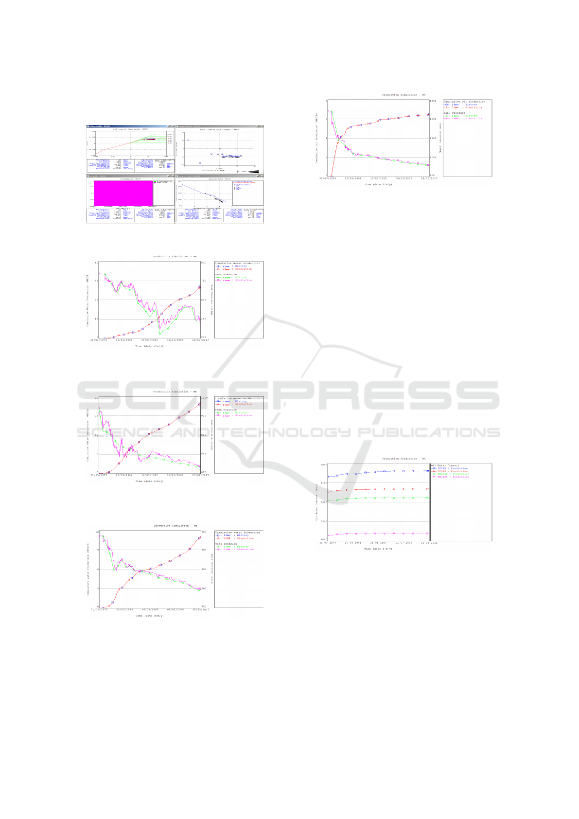
Figure 3: IPM – MBAL Initialization Output

Figure 4: Pressure and Cumulative Production History

Match from K Sand

Figure 5: Pressure and Cumulative Production History

Match from L Sand

Figure 6: Pressure and Cumulative Production History

Match from E Sand

3.6 Calibration

Material balance model calibration is needed to match

the end of history matching point with the prediction

Figure 7: Pressure and Cumulative Production History

Match from C Sand

starting point in order to make prediction more vali-

dated. In this section, pseudo-prediction will be gen-

erated by using the prediction tool. Since the goal is to

predict using tank model, a well prediction model was

not used in this case. For the constraint, history pro-

duction rate and time will be used to generate pseudo-

prediction to calibrate the model. Once both points

matched, prediction can be generated next.

3.7 Prediction

After the model already matched and validated, the

next thing is the prediction of the ﬁeld performance.

Prediction generated until the end of contract of this

ﬁeld development (August 2021). The models were

further calibrated by running pseudo-prediction for

existing sands. Results were compared with the out-

come from another method in determining the height

of OWC as shown in Fig 8.

Figure 8: OWC Prediction

4 RESULT

Various results were discussed during the study which

involved saturation reservoir with concurrently oil

production from the oil rim. Well logs will be adopted

to verify results from MBAL models. Table 3 shown

material balance results the OWC from MBAL has

compared well with the log data. For the production

forecast, it predicted using no well prediction which

ICoSET 2019 - The Second International Conference on Science, Engineering and Technology

334

assumpted the sand production rate is decline natu-

rally due to the pressure loss at the reservoir. Pre-

diction rate will be generated by software as long

the reservoir pressure and aquifer is enough to pro-

vide energies. From the result, K sand has signiﬁcant

movement of OWC, the contact moves from 2002 ft

at 1973 to 1911 ft at 2012. This 91 ft movement

in 48 years from prediction makes this sand needs

more concern due to the water production mainte-

nance. The other sand has a certain movement less

than 55 ft in 48 years.

Table 2: Predicted OOWC vs Log OOWC

Sand

MBAL

OOWC

(ft)

Log

OOWC

(ft)

Error (%)

C 2922 2925 0.103

E 2368 2366 0.085

K 2002 2002 0.000

L 2243 2246 0.134

Table 3: Predicted COWC vs Log COWC

Sand

MBAL

COWC in

2021 (ft)

MBAL

COWC in

2014(ft)

Log COWC

in 2014 (ft)

C 2922 2925 0.103

E 2368 2366 0.085

K 2002 2002 0.000

L 2243 2246 0.134

5 CONCLUSION AND

RECOMMENDATION

• Sand predictive Material Balance Models have

been proved to be a quick alternative tool to de-

termine OWC movement as reservoir simulation

in the sand analysis.

• Good surveillance acquisition data is needed to

provide input data. The accuracy of each data

needs to be concerned as pre-requisite to make

validate models.

• Sand K has the most signiﬁcant move of OWC

due to water production maintenance. It reached

91 ft in 48 years of prediction. The other sands

have certain movement below 55 ft.

• Lift tables are needed and also validated to make

well predictive models.

REFERENCES

Petroleum Experts IPM-MBAL Manual.

Campbell, R. A. and Campbell, J. M. (1978). Mineral prop-

erty economics. Petroleum Property Evaluation, 3.

Dake, L. P. (1983). Fundamentals of reservoir engineering.

Elsevier.

Daneshy, A. A. (2006). Selection and execution criteria for

water-control treatment. In SPE Symposium and Ex-

hibition on Formation Damage Control, Los Angeles.

Ghahri, P., Berthereau, G., Milner, S., Orta, M. E., Sikan-

dar, A. S., et al. (2013). Estimated ﬂuid contact using

material balance technique and volumetric calculation

improves reservoir management plan. In SPE Offshore

Europe Oil and Gas Conference and Exhibition. Soci-

ety of Petroleum Engineers.

Havlena, D. and Odeh, A. S. (1963). The material balance

as an equation of a straight line. Journal of Petroleum

Technology, pages 896–900.

Hudiman, A. and Permadi, B. Y. (2016). Analisa penentuan

laju air produksi yang optimum untuk memperlambat

water coning di lapisan tipis. JTMGB, 10(1):17–22.

Katz, B. J. and Mertani, B. (1989). Central sumatra — a

geochemical paradox. In Proc 18th Indon Pet Assoc

Ann Con, volume 1, pages 403–425, Jakarta.

Noordin, F. M., e. a. (2009). Case study: Water shut off

mechanism in small, remote platform-process & chal-

lenge. In SPE European Formation Damage Confer-

ence, pages 27–29, Netherlands.

Nwaokorie, C. and Ukakuku, I. (2012). Well predictive ma-

terial balance evaluation: A quick tool for reservoir

performance analysis. In SPE Nigerian Annual Inter-

national Conference and Exhibition, Abuja.

Stashin, K. (1989). An analytical approach to determining

oil/water contact rise at utikuma ﬁeld. In 40th Annual

Technical Meeting of The Petroleum Society, Banff.

Petro Society of CIM.

Predicting of Oil Water Contact Level using Material Balance Modeling of a Multi-tank Reservoir

335

APPENDIX

API : American Petroleum Institute

Bo : Current oil volume factor

Boi : Initial oil volume factor

Bg : Current gas volume factor

Bw : Current water volume factor

Cf : Formation compressibility

COWC : Current Oil Water Contact

Cw : Water compressibility

DST : Drill Stem Test

Et : Total expansion of ﬂuid

F : Fahrenheit

FT : Feet

Gi : Cumulative gas injection

Gp : Cumulative gas production

IOIP : Initial Oil in Place

IPM : Integrated Production Modeling

M : Gas oil Ratio

MBAL : Material Balance Modeling

Software

MSTB : Thousand Stock Tank Barrel

MMSTB : Million Stock Tank Barrel

N : Initial Oil in Place

OOIP : Original Oil in Place

OOWC : Original Oil Water Contact

OWC : Oil Water Contact

PBU : Pressure Build-Up Test

ppm : Part per Million

PSIG : Pound Square Inch Gauge

PV : Pore Volume

PVT : Pressure Volume Temperature

RCAL : Routine Core Analysis

RFT : Repeat Formation Test

Rs : Current solution gas oil ratio

Rsi : Initial solution gas oil ratio

SCAL : Special Core Analysis

SCF : Standard Cubic Feet

STB : Stock Tank Barrel

Swc : Connate water saturation

We : Water inﬂux

Wi : Cumulative water injection

Wp : Cumulative water production

ICoSET 2019 - The Second International Conference on Science, Engineering and Technology

336