Cooperative Stereo-Zoom Matching for Disparity Computation

Bo-Yang Zhuo and Huei-Yung Lin

Department of Electrical Engineering, National Chung Cheng University, Chiayi 621, Taiwan

Keywords:

Stereo Matching, Zooming, Disparity, Optical Zoom.

Abstract:

This paper investigates a stereo matching approach incorporated with the zooming information. Conventional

stereo vision algorithms take one pair of images for correspondence matching, while our proposed method

adopts two zoom lens cameras to acquire multiple stereo image pairs with zoom changes. These image se-

quences are able to provide more accurate results for stereo matching algorithms. The new framework makes

the rectiﬁed images compliant with the zoom characteristics by the deﬁnition of the relationship between

the left and right images. Our approach can be integrated with existing stereo matching algorithms under

some requirements and adjustments. In the experiments, we test the proposed framework on 2014 Middle-

bury benchmark dataset and our own zoom image dataset. The results have demonstrated the improvement of

disparity computation of the our technique.

1 INTRODUCTION

Stereo vision for machine perception is to simulate

the human visual system. When an object is closer to

the observer, the disparity between the left and right

eyes becomes larger. With this property, the stereo

vision problem can be simpliﬁed as ﬁnding the cor-

responding points within an image pair. This is an

important topic in computer vision, and aims to pro-

vide the disparity maps from the depth computation

of 3D scenes or objects. In the past few decades,

stereo matching techniques have been extensively in-

vestigated by computer vision researchers and practi-

tioners. Since the availability of Middlebury stereo

datasets (Scharstein and Szeliski, 2002) and pub-

lic benchmarks, many sophisticated algorithms have

been proposed and evaluated for the objective of de-

creasing the mismatching rate. Nevertheless, most ap-

proaches take standard rectiﬁed image pairs as inputs

and do not consider the image acquisition process of

a real camera system.

The image pair captured by a conventional stereo

vision system consists of two images taken from two

different cameras. This imaging model forms the two-

view geometry and the point correspondence relation

between the two images is restricted by the epipolar

constraint (Hartley and Zisserman, 2004). For con-

venience, the image pairs are commonly rectiﬁed so

that the epipolar lines are parallel to the image scan-

lines. The stereo matching can then be carried out ef-

ﬁciently along the one-dimensional image scanlines

at the cost of rectiﬁcation computation and image

warping. Since most existing stereo matching algo-

rithms work on rectiﬁed image pairs and do not con-

sider the image rectiﬁcation step, the investigation is

commonly focused on the matching cost rather than

the development and evaluation of the overall stereo

vision system.

In general, there are four steps adopted in stereo

matching algorithms: cost initialization, cost aggre-

gation, disparity selection and reﬁnement. The cost

initialization is a process to calculate the similarity

at the pixel level, such as the absolute difference or

cross correlation, etc. Since the cost calculated by

a pixel is not reliable, the cost aggregation consid-

ering a speciﬁc region is carried out to increase the

robustness (Hosni et al., 2011). The disparity selec-

tion usually adopts the winner-takes-all (WTA) strat-

egy which ﬁnds the lowest cost for the result. Alter-

natively, an image scaling approach with multi-block

matching and sub-pixel estimation can be used to re-

duce the error rate (Chang and Maruyama, 2018). The

reﬁnement process aims to improve the reliability us-

ing some techniques such as the left-right consistency,

matching conﬁdence, median ﬁlter, speckle ﬁlter, and

ground control points, etc.

The stereo vision research in recent years is di-

vided into two categories, the speed-oriented and

precision-oriented approaches. The speed-oriented

techniques concern about the computational efﬁ-

Zhuo, B. and Lin, H.

Cooperative Stereo-Zoom Matching for Disparity Computation.

DOI: 10.5220/0008877001570164

In Proceedings of the 15th International Joint Conference on Computer Vision, Imaging and Computer Graphics Theory and Applications (VISIGRAPP 2020) - Volume 4: VISAPP, pages

157-164

ISBN: 978-989-758-402-2; ISSN: 2184-4321

157

image

pre-processing

Get two

image pairs

Reliable point

or not

Remain stereo

matching results

Zoom matching

Getting Stereo

matching results

Yes

Cost aggregetion

Produce

disparity map

Figure 1: The system ﬂowchart of the proposed cooperative zoom-stereo framework for disparity computation.

ciency and consider the porting to hardware depen-

dent platforms such as FPGA, GPU, etc. (Chang and

Maruyama, 2018). On the other hand, the objective of

precision-oriented techniques is to increase the cor-

rectness of stereo matching results. In some recent

works, possible surface structures are used to improve

the accuracy (Park and Yoon, 2019), Kim and Kim

use the texture and edge information as the smooth-

ness constraints (Kim and Kim, 2016). In (Batsos

et al., 2018), various input scales, masks and cost

calculation methods are combined to make the algo-

rithms more robust. Moreover, learning based tech-

niques for stereo matching have shown signiﬁcant

progress in the past few years. In (

Zbontar and Le-

Cun, 2016), a method is proposed to learn a similar-

ity measure on small image patches using the con-

volutional neural network, and evaluating on KITTI

and Middlebury datasets. Seki et al. present a learn-

ing based penalties estimation method to derive the

parameters of the widely used semi-global matching

algorithm (Seki and Pollefeys, 2017). Cheng and

Lin present a matching technique based on image

bit-plane slicing and fusion (Cheng and Lin, 2015).

The bit-plane slices are used to ﬁnd stereo correspon-

dences and then combined for the ﬁnal disparity map.

These techniques have successfully reduced the cor-

respondence matching error, but at the cost of more

sophisticated hardware requirement.

In this work, a pair of zoom lens cameras are used

to capture the stereo image pairs with various focal

length settings (Chen et al., 2018). The existing or

newly developed stereo matching algorithms can be

incorporated with the proposed zoom-stereo frame-

work. A zoom rectiﬁcation method is presented to

reduce the zoom image correspondence search range.

We aggregate the matching cost of stereo and zoom

images to mitigate the unreliable matching. Our ap-

proach is able to improve the correspondence search

results with the additional zooming constraint, and

provides a robust disparity reliability check. Figure

1 shows the system ﬂowchart of the proposed stereo

with zooming technique. Two or more stereo image

pairs with various zoom factors are ﬁrst taken with

different focal length settings. An initial disparity

computation is ﬁrst carried out by the stereo image

pair acquired with the same focal length. A series of

zoom images captured from the same camera is used

for zoom matching, which is a process to identify the

point correspondences among the zoom images. The

cost aggregation combining the matching from stereo

and zoom is then performed to reﬁne the disparity

map.

2 THE APPROACH

2.1 Zoom-Stereo Framework

The scale of a scene or an object appeared in the im-

age is determined by the focal length of the camera or

the zoom factor. A vector deﬁned by the image center

and a speciﬁc point can be used to illustrate the phe-

nomenon when the focal length is changed. An ideal

zoom model can be described by the equation

and v

= λv

(1)

where v

and v

are the zoom vectors originated from

the principal point (or the image center), and λ is the

focal length ratio f

/ f

Normally, there are two types of zoom images,

one derived from digital zoom and the other acquired

with optical zoom. The former is synthesized by up-

or down-sampling the original image with interpola-

tion, and thus no additional information is generated

when magniﬁed. The optical zoom, on the other hand,

involves the actual lens movement, and the zoom im-

ages are captured with independent samples. In this

VISAPP 2020 - 15th International Conference on Computer Vision Theory and Applications

158

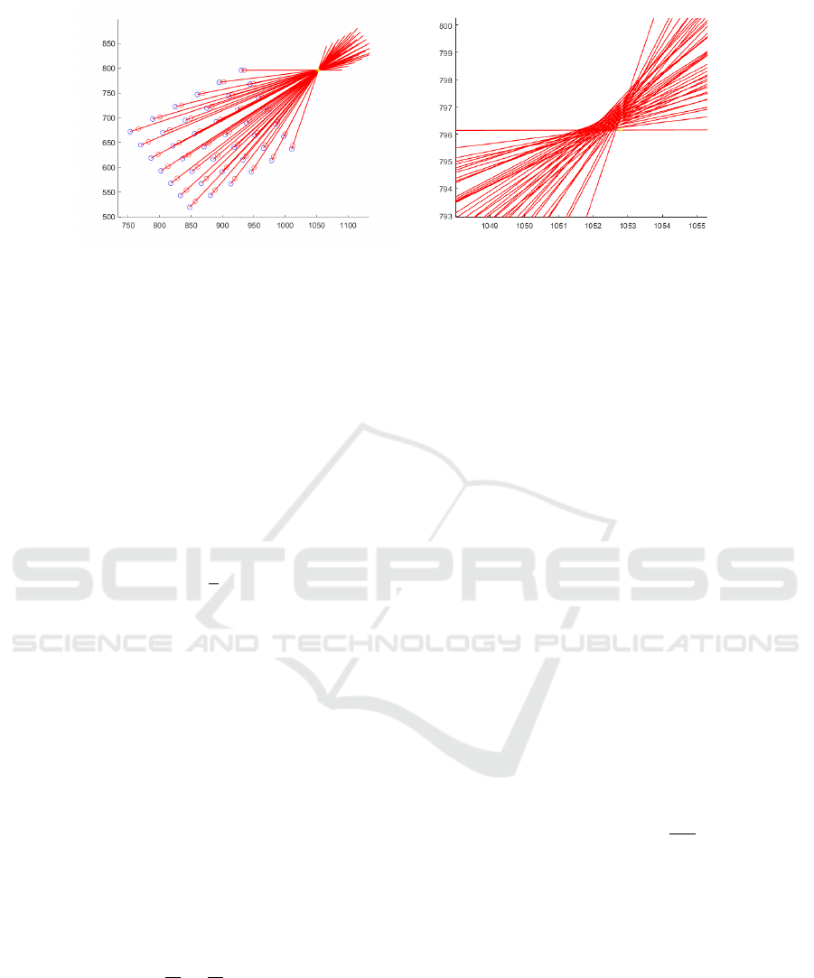
(a) Ideal zoom (b) Optical zoom

Figure 2: The red lines are connected by the same correspondences appeared in different zooms. The yellow dot is the image

center obtained from calibration.

work, the focus length is changed to acquire the zoom

images for stereo matching. One difﬁculty of optical

zoom is the change of principle point along with the

change of focus length. As illustrated in Figure 2, the

zoom vectors do not converge to a single point due to

the non-ideal lens movement of a real camera system

with optical zoom (see Figure 2(b)). This is different

from ideal case used in digital zoom (see Figure 2(a)).

In a conventional stereo vision system, the dis-

tance z of a scene point is given by

z = f

where f is the focal length of the camera, b is the

stereo baseline, and d is the stereo disparity. The

stereo baseline and focal length can be obtained by

camera calibration and used to check the disparity re-

liability by the left-right consistency (Jie et al., 2018).

Notice that a pair of zoom lens cameras is used in our

system, and several stereo image pairs are captured

at a ﬁxed location. Since the distance between the

camera and the scene does not change, additional ge-

ometric constraints can be constructed for the image

pairs. In a real camera system, the principal point will

change due to zooming (i.e., when the focal length is

adjusted). Thus, we also need to consider the base-

line change for cooperative stereo and zoom match-

ing. For a conventional stereo system setting, the dis-

parity is proportional to the stereo baseline. The re-

striction can be formulated as

(2)

where i and j represent different zoom positions for

image acquisition.

2.2 Disparity Reliability Check

For reliable stereo matching results, we need to iden-

tify the error correspondences (also called unreliable

points) in the disparity map before the calculation of

matching cost aggregation. Since the error correspon-

dences usually appear near the image edges due to the

depth discontinuity (Zhang et al., 2017), Canny edge

detection is ﬁrst carried out on the image, followed by

morphological dilation to ﬁnd the unreliable points.

The matching conﬁdence also considers the pixel lo-

cation difference between the smallest cost and the

second small cost. In our stereo with zooming ap-

proach, Equation (2) is also used to identify the unre-

liable points.

It should be noted that, Equation (2) is given in

the same world coordinate system for i and j, instead

of the image coordinates. Thus, the zoom correspon-

dence matching should be performed to align the im-

age coordinate frames. The disparity maps derived

from different zooms are then subtracted to obtain

the unreliable point map. Finally, we combine the

matching conﬁdence, edge discontinuity, and zoom-

ing to derive the error correspondences, as given by

the equations

con

[x,y] =

(

1, 1 −

1st

x,y

2nd

x,y

< τ

0, otherwise

(3)

and

R[x,y] = R

con

[x,y]∪ R

edge

[x,y]∪ R

zoom

[x,y] (4)

where τ is a user parameter and set as 0.2 in the ex-

periments. Figure 3 shows an example of the image

‘Adirondack’ in the Middlebury dataset processed by

the proposed disparity reliability check method. We

use the percentage of error correspondences marked

as unreliable points to evaluate the results, and the

values of R

con

[x,y], R

con

[x,y] ∪ R

edge

[x,y] and R[x, y]

are 46.87%, 59.47% and 71.88%, respectively.

Cooperative Stereo-Zoom Matching for Disparity Computation

159

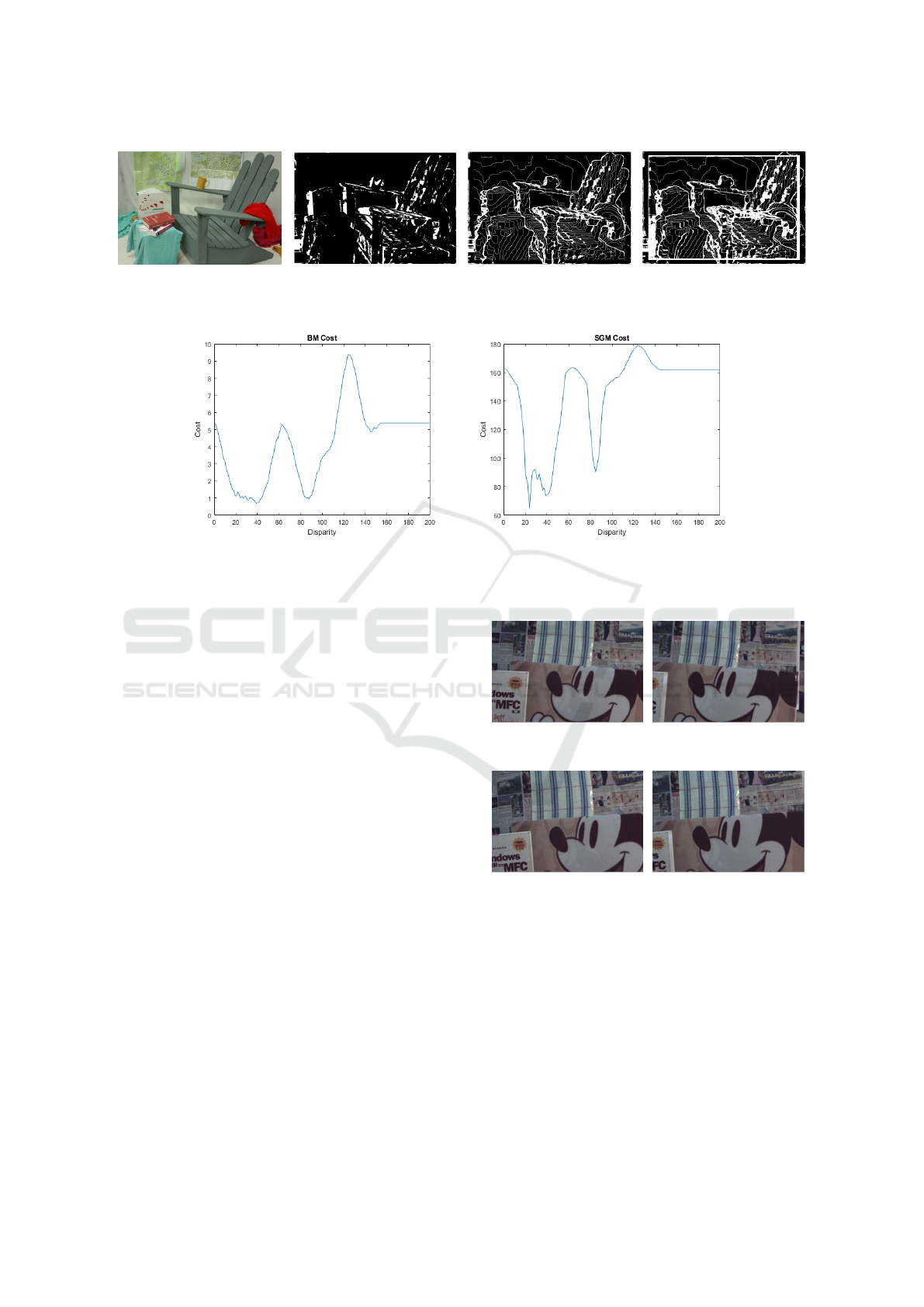
(a) Original left image (b) Error point (c) R

con

(x,y) ∪ R

edge

(x,y) (d) Result with zoom

Figure 3: The disparity reliability check on the image ‘Adirondack’ (in Middlebury 2014 dataset).

(a) BM (b) SGBM

Figure 4: The disparity cost curves for block matching (BM) and semi-global matching (SGBM).

2.3 Disparity Candidates

When calculating the disparity map, we usually pro-

vide a maximum disparity (D). The parameter D is

determined by the stereo vision system setup since

it has to be smaller than the disparity correspond-

ing to the closest scene distance perceivable by both

cameras. If all possibilities are considered for stereo

matching with different zoom images, the time com-

plexity will become O(D

). Thus, it is necessary to

choose only some speciﬁc disparities as candidates to

reduce the computation time. In general, the candi-

dates can be selected by the matching cost. However,

it might not work well for some algorithms such as

SGBM and the local minimum is used for the candi-

dates instead. Figure 4 shows the disparity cost curves

for block matching (BM) and semi-global matching

(SGBM). BM provides the more stable result com-

pared to SGBM.

2.4 Zoom Correspondence

After the main geometric construction and the match-

ing between the stereo image pair, the next problem

is to ﬁnd the correspondences among different zoom

images. For the digital zoom, the correspondence can

be obtained directly by the image scale change. How-

ever, it is not a trivial task for the optical zoom. As

(a) Zoom1 images before rectiﬁcation.

(b) Zoom2 images before rectiﬁcation.

Figure 5: Although two image are captured in the same

place, little changes of the lens will make the image rec-

tiﬁcation results different.

illustrated in Figure 5, two stereo image pairs are cap-

tured with different zoom positions. Due to the lens

movement for the zoom change, the image rectiﬁca-

tion results are not identical even a suitable scale fac-

tor is applied.

The images captured by a camera with different

zooms can thought as acquired by different cameras.

It can then be considered as multiple view geometry,

VISAPP 2020 - 15th International Conference on Computer Vision Theory and Applications

160

and the most important relationship between the im-

ages is the epipolar constraint. Except for some spe-

cial cases, the stereo matching search range can be

reduced from the 2D plane to a 1D line.

We use homography to ﬁnd the correspondences

directly for planar objects since the camera translation

is zero. It is a special case of the epipolar constraints,

and can be formulated by

= K

(R +

)Kq → sq

= Hq (5)

where q and q

are in homogeneous coordinates, R

and t is are the rotation and translation between the

cameras, n and d are the normal vector and distance of

the object with respect to the ﬁrst camera respectively,

and s is a scale factor.

To deal with the problem of the zooming prop-

erty changed by image rectiﬁcation, we use camera

calibration to establish the relationship between dif-

ferent zoom images. Since this image rectiﬁcation

only involves a rotation transformation, it can be com-

puted easily by homography. It should be noted that

the zoom property only holds under certain circum-

stances as described in Figure 2. Thus, we need to

add some constraints such as the position of the prin-

cipal point and the ﬁxed aspect ratio.

When the calibration is carried out with addi-

tional constraints, the calibration error indicated by

the re-projection error is magniﬁed as illustrated

in Table 1. The idea zoom model assumes that

two zoom images have the same principal points,

i.e. the ﬁeld-of-view changes along the optical axis.

Our calibration result is with a little difference in

rotation: (−0.05

◦

,−1.18

◦

,−0.08

◦

) and translation:

(−0.7,2.7,−1.88). This should be neglected in most

common situations (Joshi et al., 2004). For more pre-

cise results, we adopt the SIFT features (Lowe et al.,

1999) and RANSAC (Fischler and Bolles, 1981) for

the correspondence matching to calculate a new zoom

center.

2.5 Cost Aggregation

To combine the information of two zoom image pairs,

it is necessary to study how their relationship can be

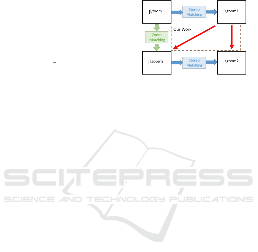
used. Figure 6 shows the concept and schematic dia-

gram of the proposed approach. The major concerns

are indicated by the red arrows since there is no guar-

antee of correspondence matching in this part. Here

we deﬁne a new cost function

Disparity =arg min

α(C

zoom1

zoom2

) + β(C

)

1 ≤ n ≤ 3,1 ≤ m ≤ 3

(6)

Figure 6: The relationship between two zoom image pairs.

The blue arrows represent the stereo matching, and the

green arrow represents the zoom correspondence.

where

= Cost(i, j,d

(i, j)),1 ≤ n ≤ 3 (7)

and

= Cost(Z

(i − d

(i, j), j), Z

− d

, j

), j

))

+Cost(Z

(i − d

(i, j), j), Z

, j

))

1 ≤ n ≤ 3,1 ≤ m ≤ 3

(8)

We only consider the pairs which are produced by the

disparity candidates, and Cost is a similarity metric

such as SSD, CT, or NCC. C

zoom1

and C

zoom2

can be

replaced by the cost given in the stereo matching al-

gorithms.

Equation (6) is based on the texture information.

In the reliability check, we use the disparity as a con-

straint. The correspondence pair produced by zoom

images are in the same place, so their distances to the

camera are the same. Thus, the cost function can in-

corporate the disparity constraint and is written as

FinalDisparity = argmin

α(C

zoom1

zoom2

)

+β(Disparity

zoom1

− Disparity

zoom2

)

1 ≤ n ≤ 3,1 ≤ m ≤ 3 (9)

where α and β are user deﬁned parameters as the pre-

vious equations.

3 EXPERIMENTS

The proposed technique is tested on the Middlebury

stereo datasets and our own dataset. Since Middle-

bury datasets do not contain zoom images, we manu-

ally synthesize the zoom images by resizing. They are

used to verify our method in the cost function eval-

uation. The stereo matching algorithms adopted in

Cooperative Stereo-Zoom Matching for Disparity Computation

161

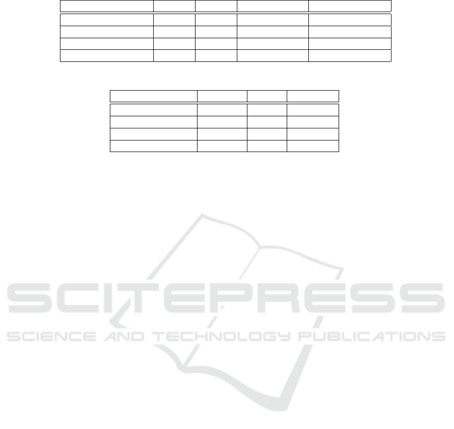
Table 1: The calibration performed under different constraints.

Condition focal X focal Y principal point reprojection error

Common 2209 2190 (988,887) (0.19,0.25)

no distortion 2962 2884 (1307,414) (0.33,0.32)

aspect=1 2166 2166 (1003,928) (0.19,0.25)

principal point ﬁxed 2243 2243 (1023.5,767.5) (0.2,0.25)

Table 2: The average minimum costs of different methods (SGBM, BM, MC-CNN).

SGBM BM MC-CNN

doll 120.236 20.92 1.1056

toy brick 120.6858 21.78 1.0581

toy brick and cup 126.8454 19.55 0.9194

toy brick and lamp 113.8195 16.643 1.3634

our framework for performance comparison are BM,

SGBM and MC-CNN. BM and SGBM run with the

window size of 13 × 13, and P

, and P

are 18 and 32,

respectively. MC-CNN uses the fast model trained by

KITTI datasets. The parameter α is ﬁxed as 1, and β is

20, 10 and 0.5 for SGBM, BM and MC-CNN, respec-

tively. The cost aggregation are tabulated in Table 2,

and the results from different methods are shown in

Tables 3–5. We choose the ‘Q’ Middlebury dataset as

the input and the evaluation method are BPR1.0.

In the cost function Equation (6), we only test CT

and NCC because the image intensity will be shifted

by the camera lens change and auto-exposure. The

results from our framework are not very signiﬁcant

when adopted to MC-CNN. This might be due to the

design of the cost function for MC-CNN training. If

only the best solution is considered during training,

it will not provide the best correspondence candidates

for the algorithm, and the normal MC-CNN has a sim-

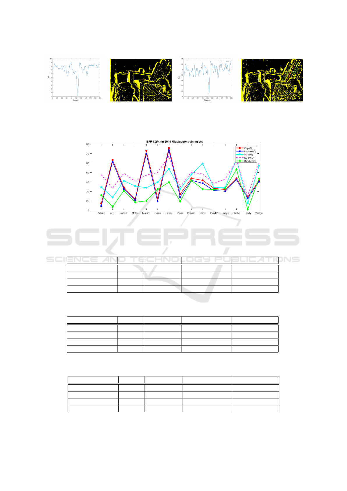
ilar process like SGBM. Figure 7 shows the results

with or without the SGBM process. There are clear

differences mainly because the basic algorithm can-

not provide the suitable candidates.

Figure 8 shows the result comparison of several

algorithms evaluated in this paper. For a fair com-

parison, we choose the same input size and remove

some machine learning based methods. We choose

SGBM+Dis as the result for comparison. The overall

performance of the framework is robust in the whole

dataset although some of them are not very signiﬁcant

mainly due to the different illumination conditions of

the left and right images.

3.1 Optical Zoom Image Dataset

We use zoom lens cameras to construct a new dataset

with ground truth. The evaluation method using our

dataset is changed to BPR2.0 because the ground truth

labeled manually is not very precise. We test the

zoom correspondence methods mentioned previously,

and test the effect of the candidate quantity. The toy

brick+BM result appears very strange. When we cal-

culate the BPR with zoom2 disparity map in BM, its

value is near to 80%. Thus, we believe that the two

initial disparity maps must have a certain level of cor-

rectness.

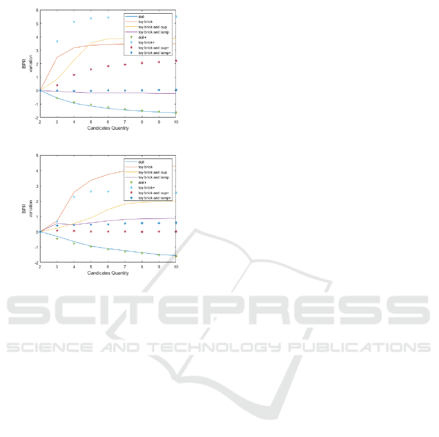
We then increase the number of disparity candi-

dates to test the relationship between the result and the

candidate quantity. In the disparity candidates, some

algorithms such as SGBM cannot just sort the cost

to choose candidates, so only MC-CNN and BM are

tested. Figure 9 shows that if we increase the number

of disparity candidates with no constraints, the results

will be unpredictable. Thus, we add a new constraint

that the correspondence pair only takes the candidates

in the top three, and the results are better improved.

MC-CNN encounters a problem that we cannot make

sure if the top three in the cost are the same as the

required candidates. The cost curve shown in Figure

7 only indicates the best disparity point. If the point

is removed the whole line will look like a horizontal

line with noise. With this test, it can be sure that the

overall framework is stable if the number of candidate

is sufﬁcient.

4 CONCLUSION

In this work, a stereo matching framework using

zoom images is proposed. With zoom image pairs, we

are able to reduce the error and the uncertain region

in the disparity map. Compared to the existing stereo

matching algorithms, our approach can improve the

disparity results with less computation. The proposed

framework can adapt to the existing local and global

methods for stereo matching, even the machine learn-

ing based matching algorithms. In the future work,

VISAPP 2020 - 15th International Conference on Computer Vision Theory and Applications

162

(a) MC-CNN+SGBM (b) Result (c) MC-CNN (d) Result

Figure 7: MC-CNN with different processes. The improvement is shown in red, and the green part indicates the incorrect

change region.

Figure 8: The result comparison of different approaches. Here we use SGBM+Dis as our result and ‘Q’ means that we use the

quarter size image as input. SGM and SGBM are different with their basic cost functions, SGM is CT and the other is SAD.

The input of SGMEPI is in full size.

Table 3: SGBM + Equation (9).

Original Homography Epipole Geometry Zoom calibration

doll 19.6503 15.2552 15.5919 15.801

toy brick 14.5528 13.3947 13.6271 13.3372

toy brick and cup 9.8251 9.2016 9.5835 9.0291

toy brick and lamp 19.6457 17.6351 17.5975 17.804

Table 4: BM + Equation (9).

Original Homography Epipole Geometry Zoom calibration

doll 25.5569 22.3145 22.3699 23.0199

toy brick 15.1138 15.7089 15.7333 15.5487

toy brick and cup 12.797 12.1638 11.7294 12.1277

toy brick and lamp 26.4771 25.8682 25.2747 25.6811

Table 5: MC-CNN (No SGBM) + Equation (9).

Original Homography Epipole Geometry Zoom calibration

doll 22.3460 20.2321 21.0419 20.4651

toy brick 18.9041 25.8092 21.7056 24.3230

toy brick and cup 11.8306 12.9873 12.8016 12.9491

toy brick and lamp 23.2376 22.8388 22.4940 22.9996

Cooperative Stereo-Zoom Matching for Disparity Computation

163

MC-CNN (No SGBM)

Figure 9: The effect of the candidate quantity, ‘+’ means

adding the constraint about the candidate order.

more investigation will be carried out to aggregate

the information for machine learning methods and the

cost computation.

REFERENCES

Batsos, K., Cai, C., and Mordohai, P. (2018). Cbmv: A

coalesced bidirectional matching volume for disparity

estimation. In Proceedings of the IEEE Conference

on Computer Vision and Pattern Recognition, pages

2060–2069.

Chang, Q. and Maruyama, T. (2018). Real-time stereo vi-

sion system: a multi-block matching on gpu. IEEE

Access, 6:42030–42046.

Chen, Y., Zhuo, B., and Lin, H. (2018). Stereo with

zooming. In 2018 IEEE International Conference on

Systems, Man, and Cybernetics (SMC), pages 2224–

2229.

Cheng, K. and Lin, H. (2015). Stereo matching with bit-

plane slicing and disparity fusion. In 2015 IEEE In-

ternational Conference on Systems, Man, and Cyber-

netics, pages 341–346.

Fischler, M. A. and Bolles, R. C. (1981). Random sample

consensus: a paradigm for model ﬁtting with appli-

cations to image analysis and automated cartography.

Communications of the ACM, 24(6):381–395.

Hartley, R. I. and Zisserman, A. (2004). Multiple View Ge-

ometry in Computer Vision. Cambridge University

Press, second edition.

Hosni, A., Bleyer, M., Rhemann, C., Gelautz, M., and

Rother, C. (2011). Real-time local stereo matching

using guided image ﬁltering. In 2011 IEEE Interna-

tional Conference on Multimedia and Expo, pages 1–

6. IEEE.

Jie, Z., Wang, P., Ling, Y., Zhao, B., Wei, Y., Feng, J.,

and Liu, W. (2018). Left-right comparative recur-

rent model for stereo matching. In Proceedings of

the IEEE Conference on Computer Vision and Pattern

Recognition, pages 3838–3846.

Joshi, M. V., Chaudhuri, S., and Panuganti, R. (2004).

Super-resolution imaging: use of zoom as a cue. Im-

age and Vision Computing, 22(14):1185–1196.

Kim, K.-R. and Kim, C.-S. (2016). Adaptive smoothness

constraints for efﬁcient stereo matching using texture

and edge information. In Image Processing (ICIP),

2016 IEEE International Conference on, pages 3429–

3433. IEEE.

Lowe, D. G. et al. (1999). Object recognition from local

scale-invariant features. In iccv, volume 99, pages

1150–1157.

Park, M.-G. and Yoon, K.-J. (2019). As-planar-as-possible

depth map estimation. Computer Vision and Image

Understanding.

Scharstein, D. and Szeliski, R. (2002). Middlebury stereo

vision page. http://vision.middlebury.edu/stereo.

Seki, A. and Pollefeys, M. (2017). Sgm-nets: Semi-global

matching with neural networks. In 2017 IEEE Con-

ference on Computer Vision and Pattern Recognition

(CVPR), pages 6640–6649.

Zbontar, J. and LeCun, Y. (2016). Stereo matching by train-

ing a convolutional neural network to compare image

patches. J. Mach. Learn. Res., 17(1):2287–2318.

Zhang, S., Xie, W., Zhang, G., Bao, H., and Kaess, M.

(2017). Robust stereo matching with surface normal

prediction. In Robotics and Automation (ICRA), 2017

IEEE International Conference on, pages 2540–2547.

IEEE.

VISAPP 2020 - 15th International Conference on Computer Vision Theory and Applications

164