Fast Local LUT Upsampling

Hiroshi Tajima, Teppei Tsubokawa, Yoshihiro Maeda and Norishige Fukushima

∗

Nagoya Institute of Technology, Japan, Tokyo University of Science, Japan

∗

https://fukushima.web.nitech.ac.jp/en/

Keywords:

Edge-preserving Filtering, Local LUT Upsampling, Acceleration, Bilateral Filtering, L

Smoothing.

Abstract:

Edge-preserving ﬁlters have been used in various applications in image processing. As the number of pixels

of digital cameras has been increasing, the computational cost becomes higher, since the order of the ﬁlters

depends on the image size. There are several acceleration approaches for the edge-preserving ﬁltering; how-

ever, most approaches reduce the dependency of ﬁltering kernel size to the processing time. In this paper, we

propose a method to accelerate the edge-preserving ﬁlters for high-resolution images. The method subsam-

ples an input image and then performs the edge-preserving ﬁltering on the subsampled image. Our method

then upsamples the subsampled image with the guidance, which is the high-resolution input images. For this

upsampling, we generate per-pixel LUTs for high-precision upsampling. Experimental results show that the

proposed method has higher performance than the conventional approaches.

1 INTRODUCTION

Edge-preserving ﬁltering smooths images while

maintaining the outline in the images. There are vari-

ous edge-preserving ﬁlters for various purposes of im-

age processing, such as bilateral ﬁltering (Tomasi and

Manduchi, 1998), non-local means ﬁltering (Buades

et al., 2005), DCT ﬁltering (Yu and Sapiro, 2011),

BM3D (Dabov et al., 2007), guided image ﬁl-

tering (He et al., 2010), domain transform ﬁlter-

ing (Gastal and Oliveira, 2011), adaptive manifold ﬁl-

tering (Gastal and Oliveira, 2012), local Laplacian ﬁl-

tering (Paris et al., 2011), weighted least square ﬁl-

tering (Levin et al., 2004), and L

smoothing (Xu

et al., 2011). The applications of the edge-preserving

ﬁlters include noise removal (Buades et al., 2005),

outline emphasis (Bae et al., 2006), high dynamic

range imaging (Durand and Dorsey, 2002), haze re-

moving (He et al., 2009), stereo matching (Hosni

et al., 2013; Matsuo et al., 2015), free viewpoint

imaging (Kodera et al., 2013), depth map enhance-

ment (Matsuo et al., 2013).

The computational cost is the main issue in the re-

search of edge-preserving ﬁltering. There are several

acceleration approaches for each ﬁlter, such as bilat-

eral ﬁltering (Durand and Dorsey, 2002; Yang et al.,

2009; Adams et al., 2010; Chaudhury et al., 2011;

Chaudhury, 2011; Chaudhury, 2013; Sugimoto and

Kamata, 2015; Sugimoto et al., 2016; Ghosh et al.,

2018; Maeda et al., 2018b; Maeda et al., 2018a; Sugi-

moto et al., 2019; Fukushima et al., 2019b), non-local

means ﬁltering (Adams et al., 2010; Fukushima et al.,

2015), local Laplacian ﬁltering (Aubry et al., 2014),

DCT ﬁltering (Fujita et al., 2015; Fukushima et al.,

2019a), guided image ﬁltering (Murooka et al., 2018;

Fukushima et al., 2018) and weighted least square ﬁl-

tering (Min et al., 2014). The computational time of

each ﬁlter, however, depends on image resolution, and

it is rapidly increasing, e.g., a camera in cellphone

even have 12M pixels. For such a high-resolution im-

age, we require more acceleration techniques.

Processing with subsampling and then upsam-

pling is the most straightforward approach to ac-

celerate image processing. This approach dramat-

ically reduces processing time; however, the accu-

racy of the approximation is also signiﬁcantly de-

creased. Subsampling loses high-frequency and large

edges in images; hence, the resulting images also

lose the information. Different from super-resolution

problems, subsampling/upsampling for acceleration

can utilize a high-resolution input image as a guid-

ance signal. Joint bilateral upsampling (Kopf et al.,

2007) and guided image upsampling (He and Sun,

2015) utilize the high-resolution image for high-

quality upsampling as extensions of joint bilateral ﬁl-

tering (Petschnigg et al., 2004; Eisemann and Durand,

2004). However, both upsampling methods are spe-

ciﬁc for accelerating bilateral ﬁltering and guided im-

age ﬁltering. More application-speciﬁc upsampling,

e.g., depth map upsampling (Fukushima et al., 2016),

improves the upsampling quality.

To accelerate arbitrary edge-preserving ﬁltering,

Tajima, H., Tsubokawa, T., Maeda, Y. and Fukushima, N.

Fast Local LUT Upsampling.

DOI: 10.5220/0008963200670075

In Proceedings of the 15th International Joint Conference on Computer Vision, Imaging and Computer Graphics Theory and Applications (VISIGRAPP 2020) - Volume 4: VISAPP, pages

67-75

ISBN: 978-989-758-402-2; ISSN: 2184-4321

Input Image

Low-resolution Input Image Low-resolution Output Image

Output Image

Subsampling

Edge-preserving Filtering

Generating

Local LUT

Reference

Output

Local LUT

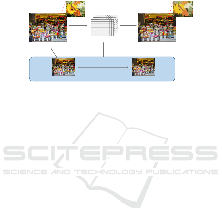
Figure 1: Local LUT upsampling: an input image is downsampled, and then the image is smoothed by arbitrary edge-

preserving ﬁltering. Next, we create per-pixel LUTs by using the correspondence between subsampled input and output

images. Finally, we convert the input image into the approximated image by the LUT.

we proposed a new upsampling method named fast

local look-up table (LUT) upsampling, which has

higher accuracy with fast computational ability than

the conventional method (Tajima et al., 2019). Fig-

ure 1 indicates an overview of our method. In

the method, edge-preserving ﬁltering, which has the

highest cost in the processing, is performed in the

downsampled domain for acceleration. Then our

method utilizes high-resolution information for accu-

rate upsampling.

This work is an extension of our previous

work (Tajima et al., 2019). The contribution of this

work is improving the computational method of per-

pixel LUT to achieve better accuracy with saving

computational time than conventional work. Also, the

proposed method is justiﬁed by state-of-the-arts up-

sampling methods (Chen et al., 2016).

2 LOCAL LUT

2.1 Concept of Local LUT

We review the concept of local LUT upsampling.

Usually, image intensity transformation by using

LUT, such as contrast enhancement, gamma correc-

tion, and tone mapping, we use a LUT for each

pixel. We call this method as global LUT. The global

LUT can represent any point-wise operations for each

pixel, but this approach cannot represent area-based

operations, such as image ﬁltering.

By contrast, our approach of the local LUT gener-

ates per-pixel LUTs. The LUT maps pixel values of

the input image to that of an image processing result.

The local LUT T

T at a pixel p

p has following relation-

ship between an input image I

I and an output image

= T

], (1)

where T [·] represents LUT reference operation. If

we have the output of edge-preserving ﬁltering, we

can easily transform the input image into the edge-

preserving result by referring the LUT. It is nonsense

that the output image is required for generating the

output image itself. Therefore, we generate the local

LUT in the subsampled image domain for accelera-

tion. The proposed method generates per-pixel LUTs

for the function from the correspondence between a

subsampled input image and its ﬁltering result.

The local LUT for each pixel is created from

neighboring pairs of low-resolution input and out-

put image around a target pixel. Luminance values

around the neighboring region have high correlations.

Also, the correlation between the output of ﬁltering

and the input image becomes high. Therefore we ag-

gregate the mapping relationship around neighboring

pixels.

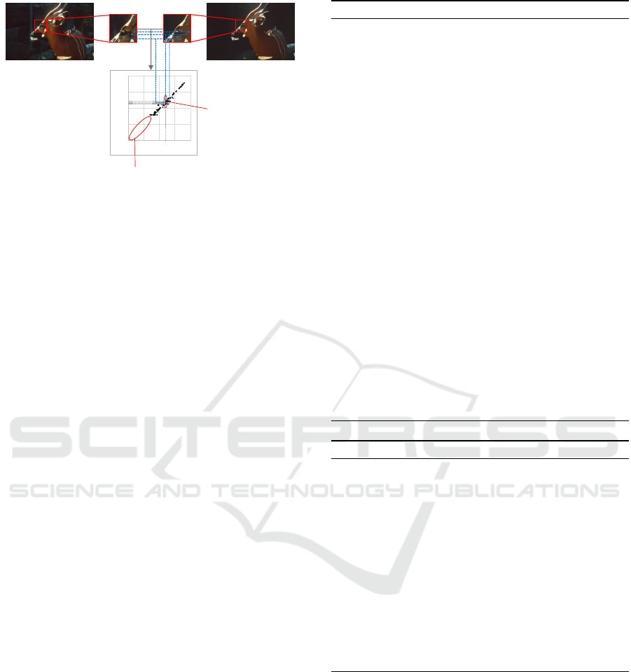
Figure 2 shows the scatter plot of intensity pair

between a local patch of an input image and a ﬁl-

tered image. The correspondence map almost repre-

sents the local LUT, but there are two issues; multiple

output candidates and gap issues. LUT requires one-

to-one mapping for each intensity of input and output,

but this scatter plot represents one-to-zero or one-to-

n matching. Our previous work (Tajima et al., 2019)

and this work solves the issues.

2.2 Conventional Approach

We shortly introduce the computing method of the lo-

cal LUT in (Tajima et al., 2019). Initially, an input

VISAPP 2020 - 15th International Conference on Computer Vision Theory and Applications

128

0 32 64 96 128

Output

Input

Gap

Multiple output candidates

I J

↓

Figure 2: Issues in generating local LUT: We make a

scatter-plot for correspondence between input and output

subsampled images in a local window. The scatter-plot al-

most represents the LUT for mapping input to output. But

there are two problems; gap and multiple-output candidates.

image I

I is subsampled to generate a low-resolution

input image I

↓

= S

I), (2)

where S

is a subsampling operator. Then, edge-

preserving ﬁltering is applied for I

↓

and the subsam-

pled output J

↓

is obtained as follows:

↓

= F(I

↓

), (3)

where F is an operator of arbitrary edge-preserving

ﬁltering. Then, we create a local LUT on a pixel from

the correspondence between I

↓

and J

↓

. Let be p

↓

the

target pixel in the subsampled images of I

↓

and J

↓

The local LUT on p

↓

is deﬁned as follows:

p↓

= Func{I

↓

, p

↓

p↓

}, (4)

where W

p↓

is a set of neighboring pixels around p

↓

Func{·} indicates each approach for generating the

local LUT.

Here, we review two conventional approaches

to generating the local LUT, which is proposed

in (Tajima et al., 2019). The ﬁrst one is the dynamic

programming approach (DP). This approach simul-

taneously solves the problems of gap and multiple-

candidates. This algorithm is shown in Algorithm 1.

In the approach, we count frequency of one-to-one

mapping of intensity between the images I

↓

and J

↓

in local window W

p↓

. Let introduce a frequency map

p↓

(s,t) on a pixel p

↓

, where s and t are an intensity

value on I

↓

and J

↓

, respectively. The frequency is

counted by gathering around a pixel W

p↓

Also, we consider quantization of the intensity for

acceleration. S

(x) is a quantization function and de-

ﬁned by:

(x) = bx/lc (5)

where l is a quantization parameter. The output of the

local LUT has 256/l dimensions. We call the number

of intensity candidates as the number of bins.

Algorithm 1: DP approach.

Input: I

↓

, J

↓

, p

↓

, W

p↓

Initialization: N = (2r +1)

Initialization: L = the number of bins

Initialization: f

p↓

(s,t) = 0|

∀s,t

Let q

↓

be a neigboring pixel ({q

1↓

, ··· , q

N↓

} ∈ W

p↓

)

For (n = 1 to N)

p↓

n↓

),S

n↓

)) + +

For (i = 1 to L − 1)

p↓

(i,0)+ = f

p↓

(i − 1, 0)

p↓

(0,i)+ = f

p↓

(0,i − 1)

For (s = 1 to L − 1)

For (t = 1 to L − 1)

= f

p↓

(s − 1,t −1) + O

= f

p↓

(s − 1,t)

= f

p↓

(s,t − 1)

p↓

(s,t) = max(C

) + f

p↓

(s,t)

index(s,t) = arg max

(m = 1, 2,3)

s = L − 1, t = L − 1

While (s ≥ 0 and t ≥ 0)

p↓

[s] = t

Switch(index(s,t))

1 : s − −, t −−

2 : s − −

3 : t − −

Algorithm 2: WTA approach.

Input: I

↓

, J

↓

, p

↓

, W

p↓

Initialization: N = (2r +1)

Initialization: L = the number of bins

Initialization: f

p↓

(s,t) = 0|

∀s,t

Let q

↓

be a neigboring pixel ({q

1↓

, ··· , q

N↓

} ∈ W

p↓

)

For (n = 1 to N)

p↓

↓

),S

↓

)) + +

For (s = 0 to L − 1)

p↓

[s] = arg max

p↓

(s,t)

For (s = 0 to L − 1)

If (T

p↓

[s] = 0)

Inter polate(T

p↓

[s])

After constructing the frequency map, we opti-

mize the result by using DP. The parameter O in Algo-

rithm 1 represents an offset value to enforce diagonal

matching. The cost function of f can be recursively

updated. After ﬁlling the cost function, we trace back

the function to determine a solid pass. Note that DP

approach ensures the monotonicity in the local LUT.

The second approach is the winner-takes-all ap-

proach (WTA). The algorithm is shown in Algo-

rithm 2. In this approach, the output value of T

p↓

[s] is

determined as the most frequent intensity in the out-

Fast Local LUT Upsampling

put image for intensity s in the input image. How-

ever, this approach still has the gap problem in the

LUT; thus, we interpolate the gap. ”Interpolate(·)” in

the algorithm indicates linearly interpolating between

the nearest existing values in bins. For the bound-

ary condition of interpolation, we set T

p↓

[0] = 0 and

p↓

[255] = 255. The solution cannot keep mono-

tonicity for the local LUT. The fact sometimes gen-

erates negative edges.

After WTA and DP, the matrix indicates one-to-

one mapping. We call this per-pixel mapping function

p↓

as local LUT. These approaches require a fre-

quency map, i.e., 2D histogram. The number of ele-

ments in the map is L

. Usually, L = 256 for no-range

downsampling case, we initialize 65536 elements per

each pixel by setting 0. By contrast, the size of the

local window is r × r, and typically r = 2, 3, 4, or

5. Thus, the size of the frequency map is dominant.

Also, the cost of memory access for more massive ar-

ray has higher than arithmetic operations in current

computers (Hennessy and Patterson, 2017).

3 PROPOSED METHOD

3.1 Fast Local LUT

In this section, we propose an acceleration method of

local LUT computation. For acceleration, we remove

the computing process of the frequency map counting

from the algorithm. We call the new approach fast

local LUT (FLL).

In FLL, we solve the multiple-candidates problem

in the local LUT computation by giving priority to the

correspondence matching. The priority is the near-

ness of distance between a target pixel position and

reference pixel position of neighborhood pixels. If

we have multiple candidates, we adopt the intensity

of the pixel where locates the nearest position from

the center of the local window. With this priority, we

can directly compute a local LUT on a pixel without

counting the frequency map.

We implemented two methods to solve the local

LUT with the nearness priority. Note that both two

methods have the same result. The ﬁrst implementa-

tion is raster scan order computation. This approach

determines the output values of the local LUT by

scanning the local window with the raster scan order.

The algorithm 3 shows this method. In this method,

we compare spatial distance of L

norm between p

↓

and q

n↓

, when T

↓

n↓

)] already has the output

value. Therefore, this method has two comparing op-

erations, i.e., NULL check and distance comparison.

Algorithm 3: FLL (Raster scan).

Input: I

↓

, J

↓

, p

↓

, W

p↓

Initialization: N = (2r +1)

Initialization: L = the number of bins

Let q

↓

be a neigboring pixel ({q

1↓

, ··· , q

N↓

} ∈ W

p↓

)

For (n = 1 to N)

distance[n] = |p

↓

−q

n↓

| //computable in advance

For (n = 1 to N)

If (T

p↓

↓

)]=NULL)

p↓

↓

)] = S

↓

)

index[S

↓

)] = distance[n]

Else

If (distance[n] ≤ index[S

↓

)])

p↓

↓

)] = S

↓

)

index[S

↓

)] = distance[n]

For (s = 0 to L − 1)

If (T

p↓

[s] = 0)

Inter polate(T

p↓

[s])

Algorithm 4: FLL (Spiral).

Input: I

↓

, J

↓

, p

↓

, W

p↓

Initialization: k = 0, N = (2r +1)

Initialization: L = the number of bins

Let q

↓

be a neigboring pixel ({q

1↓

, ··· , q

N↓

} ∈ W

p↓

)

For (n = 1 to N)

distance[n] = |p

↓

−q

n↓

| //computable in advance

For (d = 2r to 0)

For (n = 1 to N)

If (distance[n] = d)

s index[k+ +] = n //computable in advance

For (i = 1 to N)

n = s index[i]

p↓

n↓

)] = S

n↓

)

For (s = 0 to L − 1)

If (T

p↓

[s] = 0)

Inter polate(T

p↓

[s])

The second implementation is that determines out-

put values of local LUT in the spiral scanning or-

der. Generating this order, we sort the pair of input

and output intensity by the key of L

norm distance

between p

↓

and q

n↓

with descending order. Algo-

rithm 4 shows the algorithm of this method. In this

method, the value is overwritten by a new one, even

if T

↓

n↓

)] already has the output value, because

new one in the sorted order must have the nearer dis-

tance than the previous one. Therefore, there is no

comparing operation. Besides, the sorted order is

computable in advance and only computes at once;

thus, this method additionally reduces computational

time.

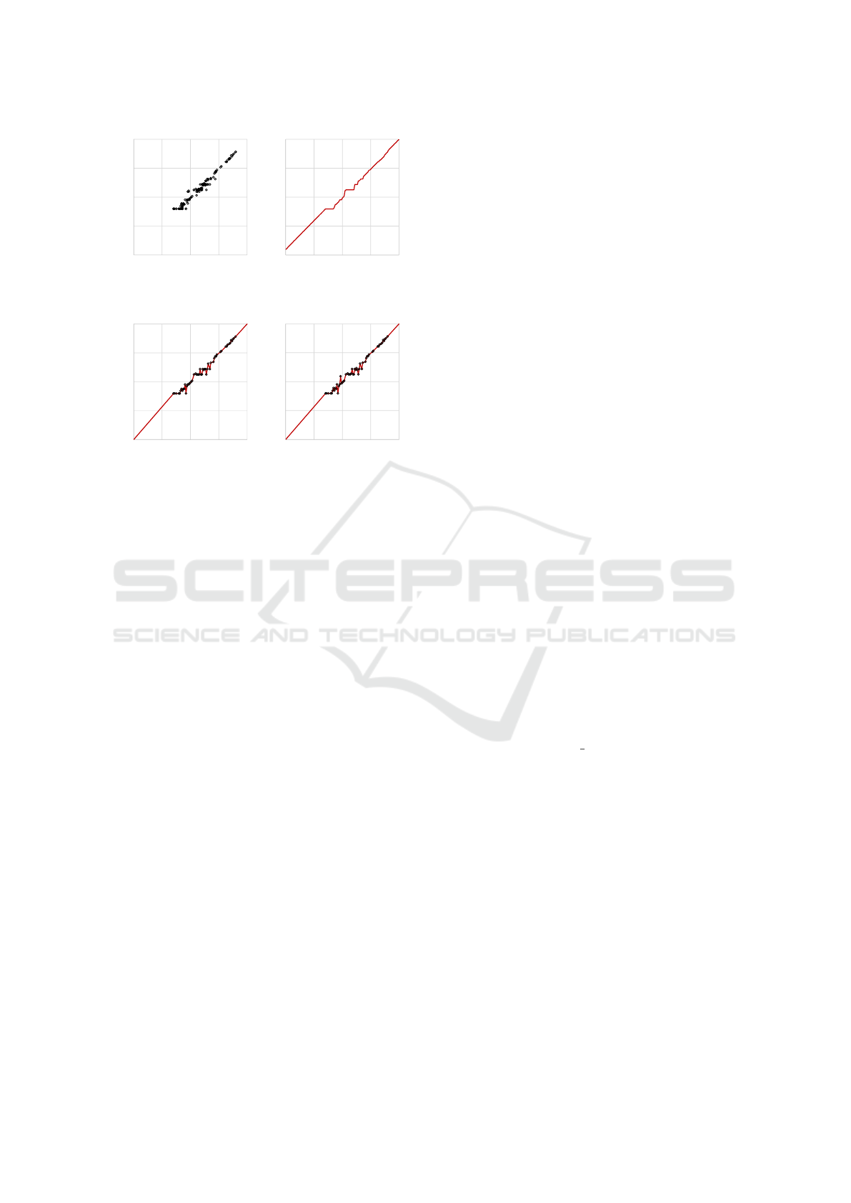
Figure 3 shows the generated local LUT of each

VISAPP 2020 - 15th International Conference on Computer Vision Theory and Applications

128

Output

Input

(a) Scatter plot

128

Output

Input

(b) DP

128

Output

Input

128

Output

Input

(d) FLL

Figure 3: Scatter plot of input and output values and results

of each approach for generating local LUT on p

p. The num-

ber of bins is 128, i.e., quantization level is l = 2. The radius

of neiboring pixels is r = 5. The subsampling rate is 1/16.

approach, i.e., DP, WTA, and FLL.

3.2 Upsampling of Local LUT

The local LUT has three-dimensional information,

such as n, p

p = (x,y); however, all elements are sub-

sampled. It has not enough to map an input image into

an output image in a high-resolution image. There-

fore, we upsample the local LUT to intensity and spa-

tial dimention. The upsampling is deﬁned as follows:

T = S

−1

↓

)), (6)

where

T and T

↓

are tensors, which gathers each lo-

cal LUT for each pixels. S

−1

(·) and S

−1

(·) are tensor

upsampling operators for the intensity and spatial do-

main of the tensors, respectively. Finally, the output

image is generated by referring to the local LUT and

input intensity of I

. The output is deﬁned by:

]. (7)

For intensity and spatial domain upsampling,

we used linear upsampling for intensity, and bilin-

ear or bicubic upsampling for spatial domain. We

call linear-bilinear pair as tri-linear upsampling, and

linear-bicubic pair as linear-bicubic upsampling.

4 EXPERIMENTAL RESULTS

We accelerated two edge-preserving ﬁlters, such as

iterative bilateral ﬁltering and L

smoothing by sub-

sampling based acceleration methods. These ﬁlters

can mostly smooth images; however, the compu-

tational cost is high. We compared the proposed

method of the local LUT upsampling with the conven-

tional method of the cubic upsampling (CU), guided

image upsampling (GIU) (He and Sun, 2015) and bi-

lateral guided upsampling (BGU) (Chen et al., 2016)

by approximation accuracy and computational time.

Also, we compared the proposed method with na

ıve

implementation, which does not subsample images,

in computational time. For the proposed method,

we also compared the fast local LUT upsampling

(FastLLU) with the conventional approach of local

LUT upsampling (LLU), which use WTA for local

LUT generation. Also, we evaluated tri-linear inter-

polation and linear-bicubic interpolation for interpo-

lating the local LUT. We utilized eight high-resolution

test images: artiﬁcial (3072 × 2048), bridge (2749 ×

4049), building (7216 × 5412), cathedral(2000 ×

3008), deer (4043 × 2641), ﬁreworks (3136 × 2352),

ﬂower (2268 × 1512), tree (6088 × 4550). We used

peak-signal noise ratio (PSNR) for accuracy evalua-

tion, and we regarded the results of the na

ıve ﬁltering

as ground truth results.

We implemented the proposed method by C++

with OpenMP parallelization. We also used Intel

IPP for the cubic upsampling, which is optimized by

AVX/AVX2. For guided image upsampling, we also

optimized by AVX/AVX2 with OpenCV functions.

For downsampling in the proposed method, we use

the nearest neighbor downsampling. For this down-

sampling, we used OpenCV and Intel IPP for the op-

eration with cv::INTER NN option. The used com-

puter was Intel Core i7 6700 (3.40 GHz) and com-

piled by Visual Studio 2017. We used r = 2 for local

LUT upsampling, iteration = 10, σ

= 10, σ

= 20,

r = 3σ

for iterative bilateral ﬁltering, and λ = 0.01

and κ = 1.5 for L

smoothing. PSNR and computa-

tional time are averages of eight high-resolution im-

ages.

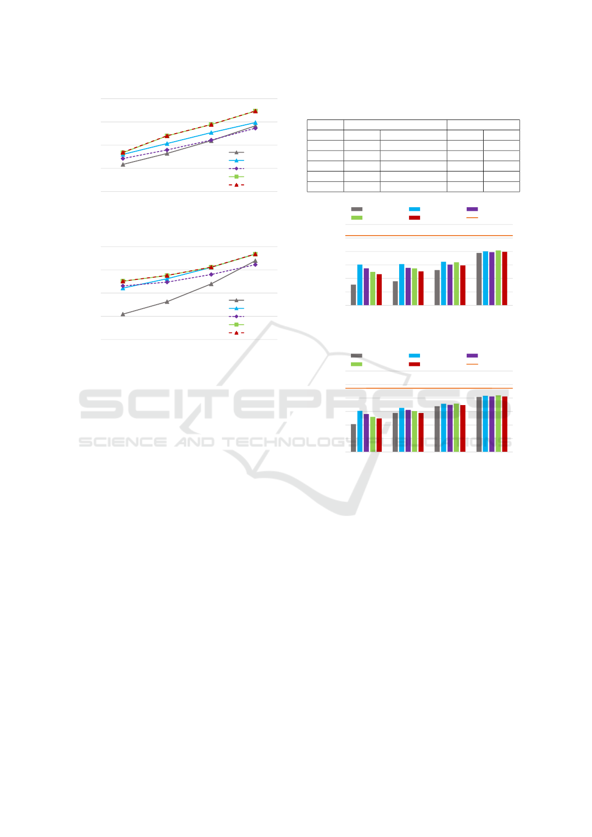
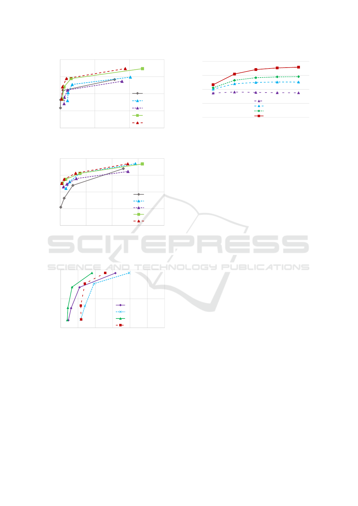
Figure 4 shows the PSNR accuracy of each ac-

celeration method for iterative bilateral ﬁltering and

smoothing, respectively. The number of bins of

the proposed method is 128. The local LUT based

methods, which are LLU and the proposed method of

fastLLU, have higher PSNR than other acceleration

methods. Note that a subsampling rate of 1/16 indi-

cates that the height and the width of images are mul-

tiplied by 1/4. Table 1 shows detail information for

LLU and fastLLU. The proposed method of fastLLU

Fast Local LUT Upsampling

1/256

1/64

1/16

1/4

PSNR [dB]

Subsampling rate

GIU

BGU

LLU

FastLLU

(a) Iterative bilateral ﬁltering

1/256

1/64

1/16

1/4

PSNR [dB]

Subsampling rate

GIU

BGU

LLU

FastLLU

(b) L

smoothing

Figure 4: Approximation accuracy of PSNR for each accel-

eration method with changing subsampling rate.

is slightly better than the conventional approach of

LLU.

Figure 5 shows the computational time of each

acceleration method for two edge-preserving ﬁlters.

The horizontal line of the graph shows the computa-

tional time of na

ıve implementation. The computa-

tional time is an average of 10 trials. The fastLLU

is the second fastest of ﬁve methods, which is ×100

faster than the na

ıve implementation when the sub-

sampling rate is 1/64. Cubic upsampling is simple

and fast, but the performance is not high.

Figure 6 shows the trade-off between the PSNR

accuracy and the computational time by changing the

subsampling rate from 1/4 to 1/256. Results show that

the fastLLU has the best performance in this trade-off

among these acceleration methods.

Figure 7 also shows the trade-off between the

PSNR accuracy and the computational time of local

LUT based methods. The result shows that the FLL

based upsampling (fastLLU) is faster than the WTA

based local LUT upsampling (LLU), and also have a

little higher PSNR. The result also shows that using

bicubic interpolation for spatial domain obtains slight

higher PSNR, though it takes a longer time.

Figure 8 show the relationship between spa-

tial/intensity subsampling rate and PSNR for iterative

bilateral ﬁltering. The spatial subsampling has a more

Table 1: Approximation accuracy of PSNR for LLU and

FastLLU (FLLU).

Iterative bilateral ﬁltering L

smoothing

LLU FLLU LLU FLLU

1/1024 26.296 26.322 31.652 31.675

1/256 28.377 28.460 32.548 32.572

1/64 31.985 32.023 33.774 33.798

1/16 34.438 34.465 35.568 35.598

1/4 37.340 37.367 38.373 38.422

100

1000

10000

100000

1000000

1/256

1/64

1/16

1/4

Time [ms]

Subsampling rate

GIU

BGU

LLU

FastLLU

naive

(a) Iterative bilateral ﬁltering

100

1000

10000

100000

1000000

1/256

1/64

1/16

1/4

Time [ms]

Subsampling rate

GIU

BGU

LLU

FastLLU

naive

(b) L

smoothing

Figure 5: Computational time for na

ıve implementation and

each acceleration method with changing subsampling rate.

signiﬁcant effect than the range subsampling.

Figures 9 and 10 depict input image and results

of each acceleration method for iterative bilateral ﬁl-

tering and L

smoothing, respectively. We omit the

result of LLU because the result is similar to the

FastLLU.

Figure 11 depict results of each approach of the

proposed method for L

smoothing.

5 CONCLUSIONS

In this paper, we proposed an acceleration method

for edge-preserving ﬁltering with image upsampling.

The local LUT upsampling has higher approximation

accuracy than conventional methods. Also, the lo-

cal LUT upsampling accelerates ×100 faster than the

VISAPP 2020 - 15th International Conference on Computer Vision Theory and Applications

5000

10000

15000

PSNR [dB]

Time [ms]

GIU

BGU

LLU

FastLLU

(a) Iterative bilateral ﬁltering

5000

10000

15000

20000

PSNR [dB]

Time [ms]

GIU

BGU

LLU

FastLLU

(b) L

smoothing

Figure 6: Changing subsampling rate performance in PSNR

w.r.t. the computational time of each acceleration method.

500

1000

1500

2000

2500

3000

PSNR [dB]

Time [ms]

WTA-tri-linear

WTA-linear-bicubic

FLL-tri-linear

FLL-linear-bicubic

Figure 7: Changing subsampling rate performance in PSNR

w.r.t. the computational time of each approach for the pro-

posed (Iterative bilateral ﬁltering).

ıve implementation. We also described that fast

LUT upsampling could obtain a higher approximation

of accuracy and faster computational time than using

the WTA approach. Also, by using bicubic interpola-

tion, the proposed method can output more accurate

results.

128

256

PSNR [dB]

Number of bins

subsampling rate : 1/256

subsampling rate : 1/64

subsampling rate : 1/16

subsampling rate : 1/4

Figure 8: Accuracy of PSNR by changing the number of lut

bins for the proposed method (Iterative bilateral ﬁltering).

ACKNOWLEDGEMENTS

This work was supported by JSPS KAKENHI

(JP17H01764, 18K18076, 19K24368).

REFERENCES

Adams, A., Baek, J., and Davis, M. A. (2010). Fast high-

dimensional ﬁltering using the permutohedral lattice.

Computer Graphics Forum, 29(2):753–762.

Aubry, M., Paris, S., Hasinoff, S. W., Kautz, J., and Durand,

F. (2014). Fast local laplacian ﬁlters: Theory and ap-

plications. ACM Transactions on Graphics, 33(5).

Bae, S., Paris, S., and Durand, F. (2006). Two-scale tone

management for photographic look. ACM Transac-

tions on Graphics, pages 637–645.

Buades, A., Coll, B., and Morel, J. M. (2005). A non-local

algorithm for image denoising. In Proc. Computer Vi-

sion and Pattern Recognition (CVPR).

Chaudhury, K. N. (2011). Constant-time ﬁltering using

shiftable kernels. IEEE Signal Processing Letters,

18(11):651–654.

Chaudhury, K. N. (2013). Acceleration of the shiftable o(1)

algorithm for bilateral ﬁltering and nonlocal means.

IEEE Transactions on Image Processing, 22(4):1291–

1300.

Chaudhury, K. N., Sage, D., and Unser, M. (2011).

Fast o(1) bilateral ﬁltering using trigonometric range

kernels. IEEE Transactions on Image Processing,

20(12):3376–3382.

Chen, J., Adams, A., Wadhwa, N., and Hasinoff, S. W.

(2016). Bilateral guided upsampling. ACM Trans.

Graph., 35(6):203:1–203:8.

Dabov, K., Foi, A., Katkovnik, V., and Egiazarian, K.

(2007). Image denoising by sparse 3-d transform-

domain collaborative ﬁltering. IEEE Transactions on

image processing, 16(8):2080–2095.

Durand, F. and Dorsey, J. (2002). Fast bilateral ﬁltering

for the display of high-dynamic-range images. ACM

Transactions on Graphics, 21(3):257–266.

Fast Local LUT Upsampling

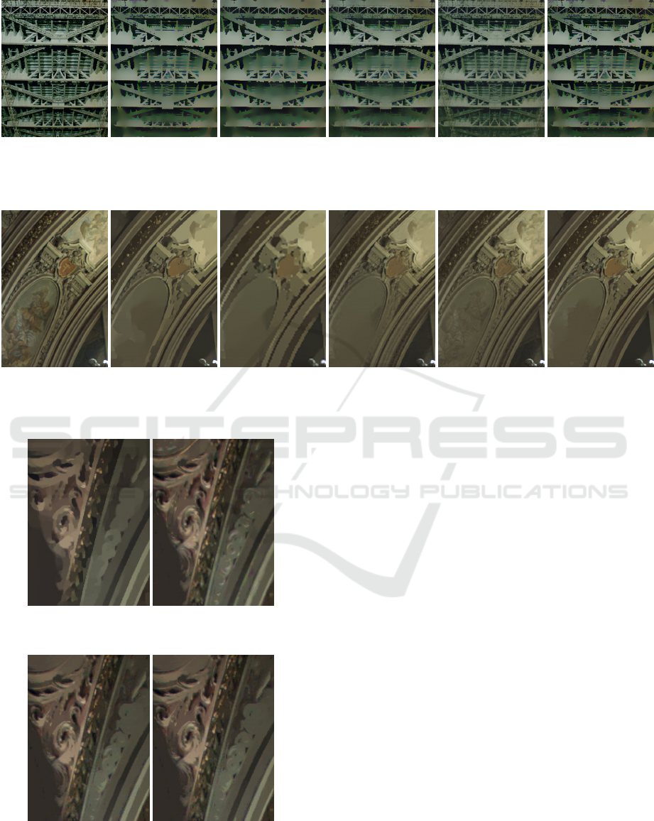
(a) input (b) na

ıve (c) cubic

28.834 dB

(d) guided

28.936 dB

(e) BGU

27.189 dB

(f) Fast LLU

30.679 dB

Figure 9: Results of iterative bilateral ﬁltering.

(a) input (b) na

ıve (c) cubic

32.038 dB

(d) guided

34.451 dB

(e) BGU

33.796 dB

(f) fast LLU

35.143 dB

Figure 10: Results of L

smoothing.

(a) na

ıve (b) DP

32.646 dB

35.077 dB

(d) FLL

35.114 dB

Figure 11: Results of each approach for the proposed.

Eisemann, E. and Durand, F. (2004). Flash photography en-

hancement via intrinsic relighting. ACM Transactions

on Graphics, 23(3):673–678.

Fujita, S., Fukushima, N., Kimura, M., and Ishibashi, Y.

(2015). Randomized redundant dct: Efﬁcient denois-

ing by using random subsampling of dct patches. In

Proc. ACM SIGGRAPH Asia 2015 Technical Briefs.

Fukushima, N., Fujita, S., and Ishibashi, Y. (2015). Switch-

ing dual kernels for separable edge-preserving ﬁl-

tering. In Proc. IEEE International Conference on

Acoustics, Speech and Signal Processing (ICASSP).

Fukushima, N., Kawasaki, Y., and Maeda, Y. (2019a). Ac-

celerating redundant dct ﬁltering for deblurring and

denoising. In IEEE International Conference on Im-

age Processing (ICIP).

Fukushima, N., Sugimoto, K., and Kamata, S. (2018).

Guided image ﬁltering with arbitrary window func-

tion. In Proc. IEEE International Conference on

Acoustics, Speech and Signal Processing (ICASSP).

Fukushima, N., Takeuchi, K., and Kojima, A. (2016). Self-

similarity matching with predictive linear upsampling

for depth map. In Proc. 3DTV-Conference.

Fukushima, N., Tsubokawa, T., and Maeda, Y. (2019b).

Vector addressing for non-sequential sampling in ﬁr

image ﬁltering. In IEEE International Conference on

Image Processing (ICIP).

Gastal, E. S. L. and Oliveira, M. M. (2011). Domain

transform for edge-aware image and video processing.

ACM Transactions on Graphics, 30(4).

Gastal, E. S. L. and Oliveira, M. M. (2012). Adaptive man-

VISAPP 2020 - 15th International Conference on Computer Vision Theory and Applications

ifolds for real-time high-dimensional ﬁltering. ACM

Transactions on Graphics, 31(4).

Ghosh, S., Nair, P., and Chaudhury, K. N. (2018). Opti-

mized fourier bilateral ﬁltering. IEEE Signal Process-

ing Letters, 25(10):1555–1559.

He, K. and Sun, J. (2015). Fast guided ﬁlter. CoRR,

abs/1505.00996.

He, K., Sun, J., and Tang, X. (2009). Single image haze

removal using dark channel prior. In Proc. Computer

Vision and Pattern Recognition (CVPR).

He, K., Sun, J., and Tang, X. (2010). Guided image ﬁl-

tering. In Proc. European Conference on Computer

Vision (ECCV).

Hennessy, J. L. and Patterson, D. A. (2017). Computer Ar-

chitecture, Sixth Edition: A Quantitative Approach.

Morgan Kaufmann Publishers Inc., San Francisco,

CA, USA, 6th edition.

Hosni, A., Rhemann, C., Bleyer, M., Rother, C., and

Gelautz, M. (2013). Fast cost-volume ﬁltering for

visual correspondence and beyond. IEEE Transac-

tions on Pattern Analysis and Machine Intelligence,

35(2):504–511.

Kodera, N., Fukushima, N., and Ishibashi, Y. (2013). Fil-

ter based alpha matting for depth image based render-

ing. In Proc. IEEE Visual Communications and Image

Processing (VCIP).

Kopf, J., Cohen, M. F., Lischinski, D., and Uyttendaele, M.

(2007). Joint bilateral upsampling. ACM Transactions

on Graphics, 26(3).

Levin, A., Lischinski, D., and Weiss, Y. (2004). Coloriza-

tion using optimization. ACM Transactions on Graph-

ics, 23(3):689–694.

Maeda, Y., Fukushima, N., and Matsuo, H. (2018a). Ef-

fective implementation of edge-preserving ﬁltering on

cpu microarchitectures. Applied Sciences, 8(10).

Maeda, Y., Fukushima, N., and Matsuo, H. (2018b). Taxon-

omy of vectorization patterns of programming for ﬁr

image ﬁlters using kernel subsampling and new one.

Applied Sciences, 8(8).

Matsuo, T., Fujita, S., Fukushima, N., and Ishibashi, Y.

(2015). Efﬁcient edge-awareness propagation via

single-map ﬁltering for edge-preserving stereo match-

ing. In Proc. SPIE, volume 9393.

Matsuo, T., Fukushima, N., and Ishibashi, Y. (2013).

Weighted joint bilateral ﬁlter with slope depth com-

pensation ﬁlter for depth map reﬁnement. In Proc.

International Conference on Computer Vision Theory

and Applications (VISAPP).

Min, D., Choi, S., Lu, J., Ham, B., Sohn, K., and Do,

M. N. (2014). Fast global image smoothing based on

weighted least squares. IEEE Transactions on Image

Processing, 23(12):5638–5653.

Murooka, Y., Maeda, Y., Nakamura, M., Sasaki, T., and

Fukushima, N. (2018). Principal component analysis

for acceleration of color guided image ﬁltering. In

Proc. International Workshop on Frontiers of Com-

puter Vision (IW-FCV).

Paris, S., Hasinoff, S. W., and Kautz, J. (2011). Local

laplacian ﬁlters: Edge-aware image processing with

a laplacian pyramid. pages 68:1–68:12.

Petschnigg, G., Agrawala, M., Hoppe, H., Szeliski, R., Co-

hen, M., and Toyama, K. (2004). Digital photography

with ﬂash and no-ﬂash image pairs. ACM Transac-

tions on Graphics, 23(3):664–672.

Sugimoto, K., Fukushima, N., and Kamata, S. (2016).

Fast bilateral ﬁlter for multichannel images via soft-

assignment coding. In Proc. Asia-Paciﬁc Signal and

Information Processing Association Annual Summit

and Conference (APSIPA).

Sugimoto, K., Fukushima, N., and Kamata, S. (2019). 200

fps constant-time bilateral ﬁlter using svd and tiling

strategy. In IEEE International Conference on Image

Processing (ICIP).

Sugimoto, K. and Kamata, S. (2015). Compressive bilat-

eral ﬁltering. IEEE Transactions on Image Process-

ing, 24(11):3357–3369.

Tajima, H., Fukushima, N., Maeda, Y., and Tsubokawa, T.

(2019). Local lut upsampling for acceleration of edge-

preserving ﬁltering.

Tomasi, C. and Manduchi, R. (1998). Bilateral ﬁltering for

gray and color images. In Proc. International Confer-

ence on Computer Vision (ICCV), pages 839–846.

Xu, L., Lu, C., Xu, Y., and Jia, J. (2011). Image smoothing

via l0 gradient minimization. ACM Transactions on

Graphics.

Yang, Q., Tan, K. H., and Ahuja, N. (2009). Real-time o

(1) bilateral ﬁltering. In Proc. Computer Vision and

Pattern Recognition (CVPR), pages 557–564.

Yu, G. and Sapiro, G. (2011). Dct image denoising: A sim-

ple and effective image denoising algorithm. Image

Processing On Line, 1:1.

Fast Local LUT Upsampling