Pursuit-evasion with Decentralized Robotic Swarm in Continuous State

Space and Action Space via Deep Reinforcement Learning

Gurpreet Singh

, Daniel M. Lofaro

and Donald Sofge

Robotics and Intelligent Systems Engineering (RISE) Laboratory, Naval Air Warfare Center Aircraft Division,

Lakehurst NJ 08733, U.S.A.

Distributed Autonomous Systems Group, U.S. Naval Research Laboratory, 4555 Overlook Ave SW,

Washington DC 20375, U.S.A.

Keywords:

Swarm Robotics, Deep Reinforcement Learning, Continuous Space, Actor Critic.

Abstract:

In this paper we address the pursuit-evasion problem using deep reinforcement learning techniques. The

goal of this project is to train each agent in a swarm of pursuers to learn a control strategy to capture the

evaders in optimal time while displaying collaborative behavior. Additional challenges addressed in this paper

include the use of continuous agent state and action spaces, and the requirement that agents in the swarm

must take actions in a decentralized fashion. Our technique builds on the actor-critic model-free Multi-Agent

Deep Deterministic Policy Gradient (MADDPG) algorithm that operates over continuous spaces. The evader

strategy is not learned and is based on Voronoi regions, which the pursuers try to minimize and the evader tries

to maximize. We assume global visibility of all agents at all times. We implement the algorithm and train the

models using Python Pytorch machine learning library. Our results show that the pursuers can learn a control

strategy to capture evaders.

1 INTRODUCTION

From ﬂocks of birds to ﬁsh schools in the sea, many

social groups in nature work together to survive and

thrive. These natural behaviors inspire humans to

mimic them with robots because robots that can coop-

erate in large numbers could achieve things that would

be difﬁcult or even impossible for a single entity. For

example, following an earthquake, a swarm of search

and rescue robots could quickly explore multiple col-

lapsed buildings looking for signs of life. Addition-

ally, areas that may be threatened by large wildﬁres

may beneﬁt from the use of swarms of drones assist-

ing the emergency services in helping track and pre-

dict the ﬁre’s spread. The characteristics from swarms

in nature that appeal to researchers are robustness,

ﬂexibility, and scalability. Swarms in nature are ro-

bust because agents in the swarm can be lost without

affecting the performance of a task the swarm as a

whole is trying to achieve. Agents can also adapt and

respond to changing work needs which makes them

ﬂexible. The scalability of swarm size is the most im-

portant characteristic because the decentralized orga-

nization of agents in swarms in nature is sustainable

with 100 or 100,000 agents.

In swarm robotics the goal is to achieve com-

plex emergent behavior from simple robots with de-

centralized control. Each robot acts based on local

perception and local coordination with neighboring

robots. There are many challenges for multi-agent

settings addressed in (Nguyen et al., 2018), such

as non-stationary environments, partial observability,

and continuous action spaces. When dealing with

non-stationary environments, where the underlying

model of the environment changes over time, agents

usually have to continually re-adapt themselves to the

changing dynamics of the environment. This causes

two problems: 1) the time for relearning how to

behave makes the performance drop during the re-

adjustment phase; and 2) the system, when learning

a new optimal policy, forgets the old one, and conse-

quently makes the relearning process necessary even

for dynamics which have already been experienced.

There are cases when agents only have partial observ-

ability of the environment. In other words, complete

information of states pertaining to the environment is

not known to the agents when they interact with the

environment. In such situations the agents observe

partial information about the environment and need

to make the best decision during each time step. An-

226

Singh, G., Lofaro, D. and Sofge, D.

Pursuit-evasion with Decentralized Robotic Swarm in Continuous State Space and Action Space via Deep Reinforcement Learning.

DOI: 10.5220/0008971502260233

In Proceedings of the 12th International Conference on Agents and Artiﬁcial Intelligence (ICAART 2020) - Volume 1, pages 226-233

ISBN: 978-989-758-395-7; ISSN: 2184-433X

other challenge is that agents can operate in discrete

action space (e.g., up, down, left, right), or continu-

ous action space (e.g., velocity). The complexity of

the problem increases when agents have continuous

actions because large action spaces are difﬁcult to ex-

plore efﬁciently and can make training intractable.

In this work we consider the pursuit-evasion or

predator-prey problem and use a deep reinforcement

learning technique to solve this problem. Pursuit-

evasion is a problem where a group of agents col-

lectively try to capture one or multiple evaders while

the evaders try to avoid getting caught. Our goal is

to train agents to make decentralized decisions and

display swarm-like behavior. For our approach we

use the Multi-Agent DDPG (MADDPG) algorithm

introduced by (Lowe et al., 2017). MADDPG ex-

tends DDPG (Lillicrap et al., 2015) to the multi-agent

setting during training, potentially resulting in much

richer behavior between agents. This is an actor-critic

approach. This paper describes a centralized multi-

agent training algorithm leading to decentralized in-

dividual policies. Each agent has access to all other

agents’ state observations and actions during critic

training, but tries to predict its own actions with only

its own state observations during execution.

2 METHODOLOGY

In this section we give an intuitive explanation of the

theory behind reinforcement learning and then intro-

duce the recent developments in deep reinforcement

learning implemented herein.

2.1 Reinforcement Learning

Reinforcement Learning (RL) is a goal-oriented

reward-based learning technique. In RL agents inter-

act with an environment in discrete time-steps and at

each time-step, the agent observes the environment,

then takes an action and receives a numeric reward

based on the action. The goal of RL is to learn a good

strategy (policy) for the agent from experimental tri-

als and relatively simple feedback received (reward

signal). With the learned strategy, the agent is able to

actively adapt to the environment to maximize future

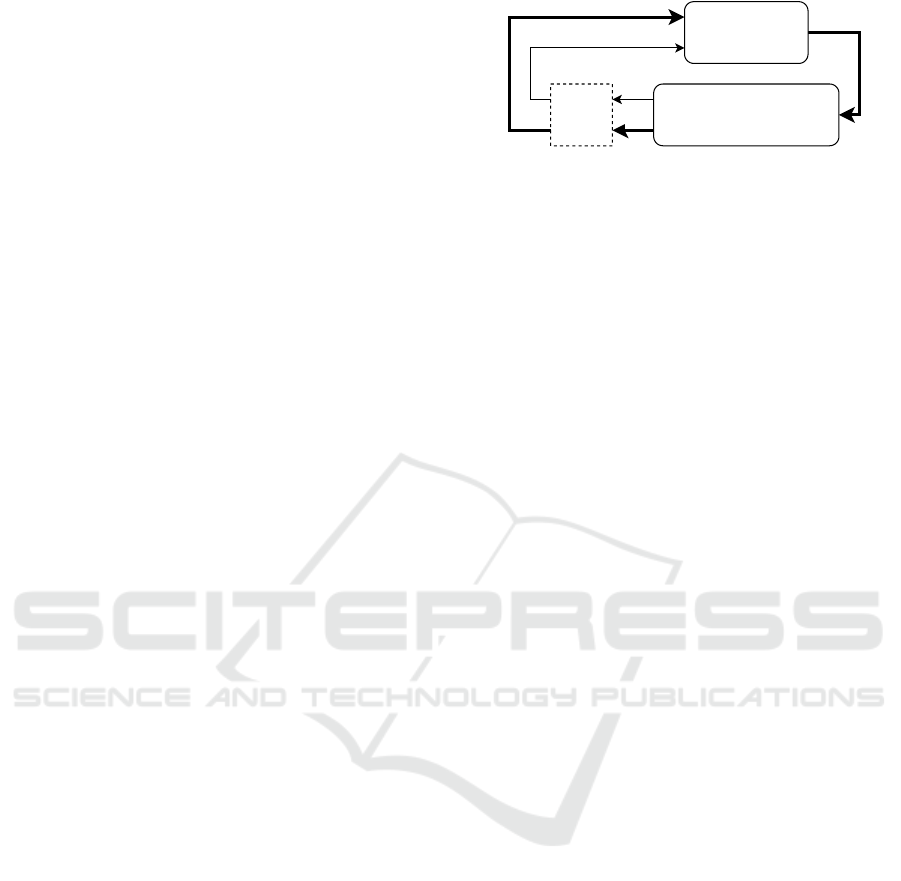
rewards. Figure 1 shows the RL framework.

The RL framework can be formalized using a

Markov Decision Process (MDP) deﬁned by a set of

states S, a set of actions A, an initial state distribution

p(s

), a reward function r : S x A 7→ R, transition prob-

abilities P(s

t+1

, a

), and a discount factor γ. The

agents take action based on their policy denoted by

Reward

Action

Agent

t+1

Environment

sampling

t+1

State

Figure 1: Reinforcement learning framework simpliﬁed

system diagram based on (Sutton and Barto, 2018).

parameterized by θ, which can be either determin-

istic or stochastic. Deterministic policies are used in

environments where for every state you have a clear

deﬁned action you will take. Stochastic policies are

used in environments where for every state, for you to

take an action, you draw a sample from possible ac-

tions that follow a distribution. A value function mea-

sures the goodness of a state or how rewarding a state

or action is by predicting the future reward. The goal

for the agent is to learn an optimal policy that tells it

which actions to take in order to maximize its own to-

tal expected reward R

∑

t=0

, where 0 < γ < 1.

The discount factor penalizes the rewards in the future

because future rewards have higher uncertainty.

To learn an optimal policy, Richard Bellman, an

American applied mathematician, derived the Bell-

man equations which allowed us to start solving

MDPs. He made use of the state-value function de-

noted by:

(s, a) =

= s] (1)

and the action-value function denoted by

(s, a) =

= s, a

= a] (2)

to derive the Bellman equations. The state-value func-

tion speciﬁes the expected return of a state s

when

following an optimal policy, whereas the action-value

function speciﬁes the expected return when choosing

action a

in state s

and following an optimal policy.

Once we have the optimal value functions, then we

can obtain the optimal policy that satisﬁes the Bell-

man optimality equations given by:

∗

(s) = max

∈A

∑

P(s

, r|s, a)[r + γV

∗

)] (3)

∗

(s, a) =

∑

P(s

, r|s, a)[r + max

∈A

∗

, a

)] (4)

The common approaches to RL are Dynamic

Programming (DP), Monte Carlo (MC) methods,

Temporal-Difference (TD) learning, and Policy Gra-

dient (PG) methods. If we have complete knowl-

edge of the environment or all the MDP variables,

following Bellman equations, we can use DP to iter-

atively evaluate value functions and improve the pol-

icy. DP methods are known as model-based methods

Pursuit-evasion with Decentralized Robotic Swarm in Continuous State Space and Action Space via Deep Reinforcement Learning

227

Pass State

Experience to Memory

Agent

Sample Experience

Memory

Random Action

Actor

Actor (target)

Critic

Critic (target)

Train Actor and Critic

Actor

Critic

Replay Buffer

Agent 1

Actor

Critic

Replay Buffer

Agent 2

MADDPG Training Phase

State

Linear

ReLU

Linear

ReLU

Tanh

Action

Actor

States

(agent 1, agent 2, ... , agent n)

Critc

Linear

ReLU

Linear

ReLU

Linear

Q-Value

Actions

(agent 1, agent 2, ... , agent n)

MADDPG ExecutionDDPG Actor-Critic Architecture

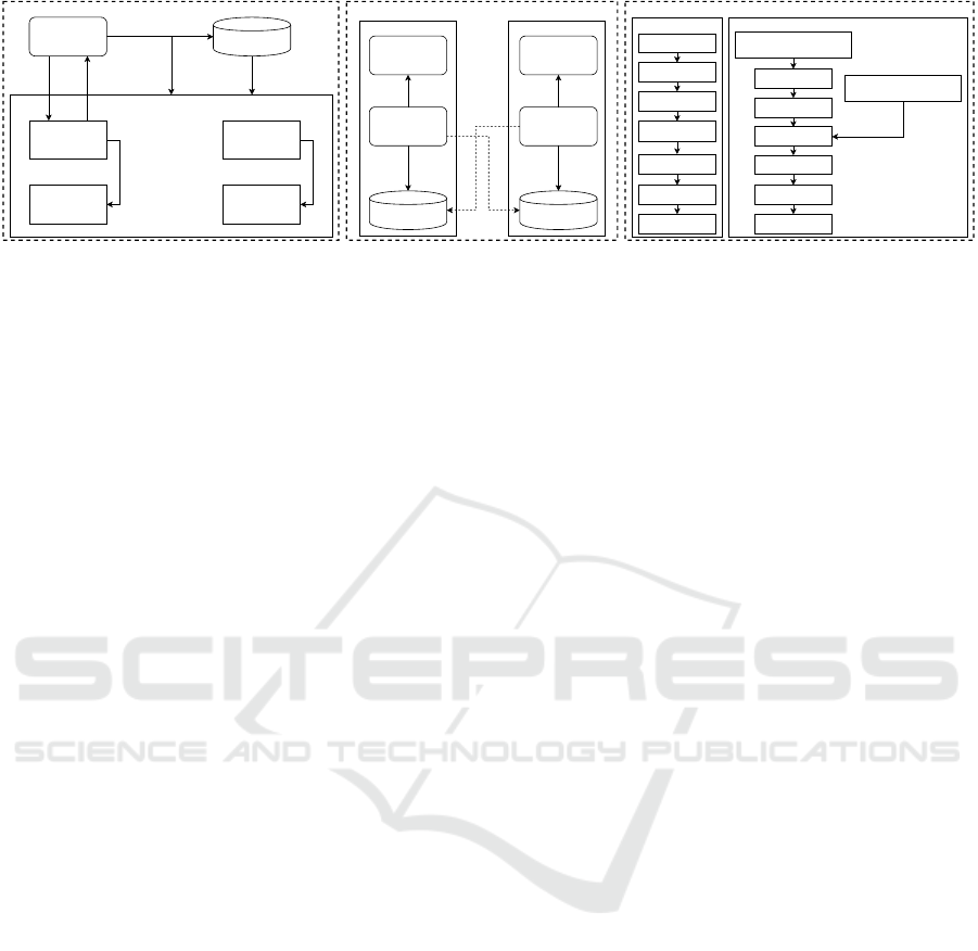
Figure 2: (LEFT): Block diagram of the Actor-Critic architecture used in the DDPG algorithm. Here an agent is trained

for a ﬁxed number of episodes and time steps. For each time step in an episode: choose an action for the given state; take

an action and receive the next state, reward, and completion status (whether the episode is ﬁnished); store the current state,

action, next state, reward, and completion status in a buffer; sample random batch of experiences; and train Actor and Critic

networks by sampling experiences from replay buffer and minimizing a loss function. Note: Both models (Actor and Critic)

get better in their own roles as time passes. (CENTER): Centralized training phase for multi-agent implementation of DDPG

(i.e. MADDPG). (RIGHT): decentralized execution of MADDPG. The MADDPG algorithm uses centralized training and

decentralized execution. Each action from the agent is used only during the training phase. During execution, the policy

network returns the actions for given states. A key improvement over the DDPG approach is that it shares the actions taken

by all agents to train each agent.

because we have complete knowledge of the environ-

ment. However, in most cases we do not know the

P(s

, r|s, a) or R(s, a), so we cannot solve MDPs by di-

rectly using the Bellman equations. This is where MC

methods become helpful. MC methods are model-

free and learn directly from episodes of experience

without any prior knowledge of MDP transition func-

tions P(s

, r|s, a) and reward functions R(s, a). How-

ever, this can only be applied to episodic MDPs be-

cause an episode has to terminate before we can

calculate any returns. Here, we do not do update

estimates after every action, but rather after every

episode. TD learning is a combination of DP and MC

methods. Like MC methods, TD methods are model-

free, meaning these methods can learn from episodes

with no prior knowledge of the environment. Like DP,

TD methods update estimates iteratively based in part

on other learned estimates, without waiting for the ﬁ-

nal outcome.

2.2 Q-Learning

Q-Learning (Watkins and Dayan, 1992) is an off pol-

icy RL algorithm that seeks to ﬁnd the best action to

take given the current state. It learns the action-value

function, Q

(s, a), by building a Q-table that stores

Q-values for all possible combinations of state and

action (s, a). The action-value function (Q-function)

takes two inputs: state and action. It returns the Q-

value (expected future reward) of that action at that

state. The Q-values are iteratively updated as we ex-

plore the environment by using the Bellman equation:

Q(s, a) ← Q(s, a) + α[r

t+1

+ γ max

Q(s

t+1

, a) − Q(s

, a

)]

(5)

2.3 Deep Q-Networks (DQN)

Theoretically, we can memorize the Q-table for all

state-action pairs in Q-learning. However, it quickly

becomes computationally infeasible when the state

and action are large discrete or continuous spaces.

Thus we have to use function approximators (e.g.

neural networks), to approximate Q-values. We can

estimate the Q-function by a supervised learning al-

gorithm with the input and output for the training

given by the reinforcement learning algorithm. The

loss function that drives the function approximator to

output the correct Q-values parameterized by learning

parameters θ is given by:

L(s

, a

, r

t+1

, s

t+1

, θ) =

t+1

+ γmax

Q(s

t+1

, a;θ) − Q(s

, a

;θ))

(6)

DQN, introduced by DeepMind (Mnih et al.,

2013), was the ﬁrst breakthrough in the fusion of RL

and Deep Learning. It used neural networks to ap-

proximate Q-values and showed that deep learning

with convolutional layers can enable reinforcement

learning algorithms to successfully learn to play Atari

2600 games. An improved version of DQN was in-

troduced in (Mnih et al., 2015) that was able to use

direct training from pixels to actions to play 49 differ-

ent Atari games without the need to change the hyper-

parameters of the network. The performance on Atari

games was impressive, as the learned policies were

often able to outperform human players. The only

input used for training the networks was the pixel im-

ages and the game score.

Neural networks are nonlinear function approxi-

mators and Q-learning suffers from instability and di-

ICAART 2020 - 12th International Conference on Agents and Artiﬁcial Intelligence

228

vergence when combined with a nonlinear Q-value

function approximation. The loss function above in-

cludes the θ parameter twice, which would make the

learning unstable. Q(s

t+1

, a;θ), which is the fore-

sight into the future, should now depend on the θ.

The DQN training method therefore introduces a tar-

get Q-network that copies the parameters from the

trained Q-network only after several hundred or sev-

eral thousand training steps and thus does not change

rapidly and enables the algorithm to learn stable long

term dependencies (Mnih et al., 2015). The loss func-

tion changes to:

L(s

, a

, r

t+1

, s

t+1

, θ, θ

−

) = (r

t+1

γmax

Q(s

t+1

, a;θ

−

) − Q(s

, a

;θ))

(7)

Using simple gradient descent on the loss function

with the target network can still lead to unstable train-

ing. DQN uses a variant of stochastic gradient descent

on the loss function and experience replay memory

to store the training examples. The experience replay

memory stores transitions between states sampled in

the past, and also memorizes the corresponding ac-

tions and rewards to correctly calculate the loss at ev-

ery time step in the future. Thus, the memory consists

of samples (s

, a

, r

i+1

, s

i+1

) for each recorded time

step. The idea behind stochastic gradient descent is

to use random samples of relatively few training ex-

amples from the experience replay buffer to estimate

the expectation of the true training error. When the

examples are sampled from very different time steps

and were generated under different conditions, they

can be sufﬁcient to provide a good estimate of the true

training error with relatively low variance.

To summarize, there are two processes that are

happening in the DQN algorithm. We sample the en-

vironment where we perform actions and store the

observed experience-tuples in the experience replay

memory. Next, we select a small batch of experience-

tuples randomly and learn from them using a gradient

descent update step.

2.4 Policy Gradients (PG)

Using Q-Learning and DQN, it is possible to derive

reasonably performing policies from good estimates

of value functions. However, policies derived from

value functions search over a discrete number of Q-

values to ﬁnd the best action, so it is not possible to

directly obtain policies that output continuous actions.

The policy gradient methods update the policy param-

eters at each step in the direction of an estimate of the

gradient of performance, ∇

J(π

), with respect to the

policy parameters. The fundamental result that under-

lies policy gradient methods is the Policy Gradient

Theorem given by:

∇

J(π

) =

s∼ρ

,a∼π

[∇

logπ

(a|s)Q

(s, a)] (8)

2.5 Deterministic Policy Gradient

(DPG)

The deterministic policy gradient method was derived

in (Silver et al., 2014). Given a deterministic policy

parameterized by θ, and a discounted state distribu-

tion, ρ

(s), induced by the policy, a performance ob-

jective function J(µ

) can be deﬁned as the expected

reward under the state distribution.

J(µ

) =

s∼ρ

[r(s, µ

(s))] (9)

and (Silver et al., 2014) proved that the gradient of

this objective function is given by:

∇

J(µ

) =

s∼ρ

[∇

(s)∇

(s, a)|

a=µ

(s)

] (10)

2.6 Deep Deterministic Policy Gradient

(DDPG)

DDPG (Lillicrap et al., 2015) combines DPG with a

DQN to obtain the deep deterministic policy gradient

(DDPG) algorithm. It uses an Actor-Critic architec-

ture to learn both the value function and the policy,

since knowing the value function can assist the policy

update. Actor and Critic are two neural network mod-

els. The Critic updates the value function parameters,

w, and depending on the algorithm it could represent

the action-value Q

(a|s) or state-value V

(s). The

Actor updates the policy parameters θ for π

(a|s), in

the direction suggested by the Critic. A block dia-

gram of the DDPG actor-critic method can be seen in

Figure 2.

In DDPG the agent is trained for a ﬁxed number

of episodes and a ﬁxed number of time-steps in each

episode. In each time-step in each episode, the agent

chooses an action for the given state and takes the ac-

tion to receive a reward. The agent will store the expe-

rience, which consists of the current state, action, next

state, and reward, in the replay memory. Afterward,

the agent will sample a random batch of experiences

to train the Actor and the Critic. In training, the Actor

network takes states as input and returns the actions,

whereas the Critic network takes states and actions as

input and returns the values. Like DQN, the DDPG

algorithm uses target networks for both the Actor and

the Critic. The critic loss is given by:

L =

∑

− Q(s

, a

|θ

))

(11)

Pursuit-evasion with Decentralized Robotic Swarm in Continuous State Space and Action Space via Deep Reinforcement Learning

229

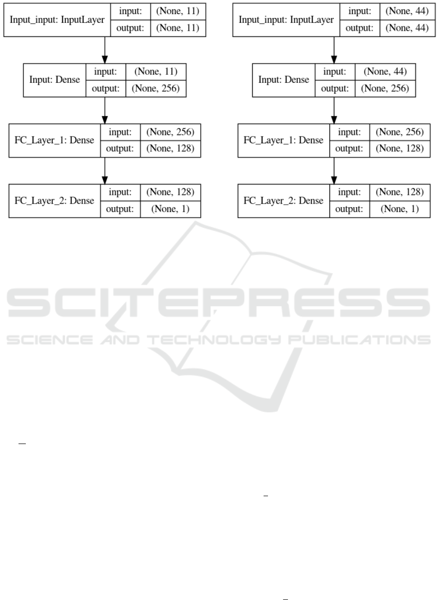
Figure 3: (LEFT): Actor (agent) model that the neural network uses for the MADDPG algorithm. Note the numbers of inputs

and outputs on the input layer and the dense layer. (RIGHT): Critic model that the neural network uses for the MADDPG

algorithm. Note how the numbers of inputs and outputs on the input layer and the dense layer are different from that of the

Actor model.

This is the average of squared differences between

the target action-value and the expected action-value

where the expected action-value is given by the lo-

cal Critic network that takes state and action as input.

The target action-value is calculated as:

= r

+ γQ

i+1

, µ

i+1

|θ

)|θ

) (12)

This calculates the target estimate by adding the re-

ward and discounted action-value where the target

critic network takes states and actions as input and

returns the action-values. The Actor is updated using

sampled policy gradient.

∇

J ≈

∑

∇

Q(s, a|θ

a=µ(s

)

s=s

∇

µ(s|θ

s=s

(13)

This is the average of action-values given by the lo-

cal Critic network that takes states and actions as in-

put where the action is estimated by the local Ac-

tor network that takes states as input. In contrast to

DQN, the target networks are updated after each gra-

dient step to slowly replicate the changes made to the

trained networks.

2.7 Multi-Agent Deep Deterministic

Policy Gradient (MADDPG)

(Lowe et al., 2017) proposed the multi-agent deep

deterministic policy gradient (MADDPG) algorithm

which extended DDPG to an environment where mul-

tiple agents coordinate to complete tasks. When the

environment has multiple agents, training agents in-

dependently does not work well because the agents

are independently updating their policies as learning

progresses and this causes the environment to appear

non-stationary from the viewpoint of a single agent.

MADDPG was designed for handling the problem of

non-stationarity. It adopts the framework of a cen-

tralized Critic training and a decentralized execution

approach. In this approach all agents have access to

all other agents’ state observations and actions during

Critic training, but during execution each agent pre-

dicts the action based on its own state. This way the

environment becomes stationary from the viewpoint

of all the agents.

The Actor policy gradient with parameter θ is

given by:

∇

J ≈

∑

∇

)∇

· Q

, a

, . . . , a

)



=µ

)

(14)

where D is the memory buffer for experience re-

play containing the tuples (x, x

, a

, ..., a

, r

, ..., r

)

of recording experiences from all the agents. The cen-

tralized Critic function is updated by minimizing the

loss function:

L(θ

) =

∑



− Q

, a

, . . . , a

)



(15)

ICAART 2020 - 12th International Conference on Agents and Artiﬁcial Intelligence

230

Table 1: Hyperparameters.

Params Value Description

γ 0.99 Discount Factor

τ 0.1 Soft update of target pa-

rameters

Actor FC1 256 Input channels for actor

fully connected hidden

layer 1

Actor FC2 128 Input channels for actor

fully connected hidden

layer 2

Critic FC1 256 Input channels for critic

fully connected hidden

layer 1

Critic FC2 128 Input channels for critic

fully connected hidden

layer 2

Actor

Learning

Rate

0.0001 Learning rate for actor

Adam optimizer

Critic

Learning

Rate

0.0001 Learning rate for critic

Adam optimizer

Batch Size 256 Number of episodes to

optimize at the same

time

Experience

Replay

Memory

Size

10M Size of the replay buffer

that stores experiences

Episodes 2048 Number of episodes

Episode

Length

256 Length of each episode

where

= r

+ γQ

, a

, . . . , a

)



=µ

)

(16)

3 TESTS AND RESULTS

We applied the MADDPG algorithm to the pursuit-

evasion task using a simulation environment provided

by Lincoln Centre for Autonomous Systems Research

(L-CAS) (H

uttenrauch et al., 2018). In this simulation

environment the agents are point robots with a unicy-

cle model. Note: the simulation environment is open-

source and available online

. The state of an agent is

given by:

Lincoln Centre for Autonomous Systems Re-

search (L-CAS): Deep RL for Swarm Systems:

https://github.com/LCAS/deep rl for swarms

= [x

, y

, φ

] ∈ S = {[x, y, φ] ∈ R

0 ≤ x ≤ x

max

, 0 ≤ y ≤ y

max

, 0 ≤ φ ≤ 2π}

(17)

Listing 1: Implementation of the MADDPG Algorithm

from (Lowe et al., 2017).

f o r e p i s o d e = 1 t o M do

I n i t i a l i z e a random p r o c e s s N f o r

a c t i o n e x p l o r a t i o n

R e ce i v e i n i t i a l s t a t e x

f o r t = 1 t o max −episode − length do

f o r eac h a g e n t i , s e l e c t a c t i o n

= µ

) + N

w . r . t . t h e

c u r r e n t p o l i c y and

e x p l o r a t i o n

E x ec u t e a c t i o n s a = (a

, .. . , a

)

and o b s e r v e rew a rd r

and new s t a t e x

S t o r e (x, a, r, x

) i n r e p l a y

b u f f e r D

x ← x

f o r a g e n t i = 1 to N

Sampl e a random m i n i b a t c h o f

S s a m p les (x

, a

, r

, x

)

fro m D

S e t y

= r

+ γQ

, a

, .. . , a

=µ

)

Up da te c r i t i c by m i n i mizi n g

t h e l o s s

L(θ

) =

∑



− Q

, a

, .. . , a

)



Up da te a c t o r u s i n g t h e

sa m pl ed p o l i c y g r a d i e n t s :

∇

J ≈

∑

∇

)∇

, a

, .. . , a

)



=µ

)

end f o r

Up da te t a r g e t n et w ork

p a r a m e t e r s f o r eac h a g e n t i :

← τθ

+ (1 − τ)θ

end f o r

The linear and angular velocities can be controlled by

the agents. The kinematics model is given by:

˙x =vcosφ

˙y =vsinφ

φ =ω

(18)

The environment is enclosed with x

max

= 100 and

max

= 100. The evader agents are 2x faster than the

pursuers. The max values for the linear and angular

velocities for the pursuer agents is in the range [−1, 1].

However, for the evader agents, the range is [−2, 2].

We keep the linear velocity constant for all the agents

so that our model only has to predict a single continu-

ous variable, angular velocity. The reward function is

expressed in terms of the distance to the closest pur-

suer,

Pursuit-evasion with Decentralized Robotic Swarm in Continuous State Space and Action Space via Deep Reinforcement Learning

231

Evader

Pursuers

Capture

(Start)

(End)

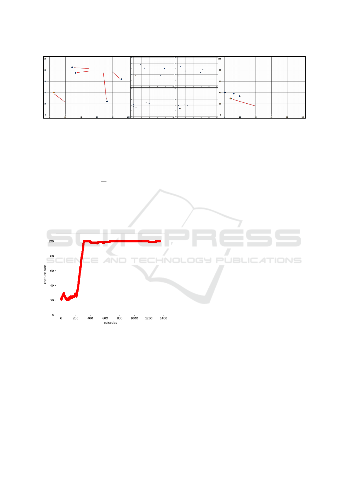
Figure 4: Experiment running in the simulation environment. Four pursuer agents successfully learn how to capture an evader

agent. The simulator used is the Deep RL for Swarm Systems by the Lincoln Centre for Autonomous Systems Research

(L-CAS). In this simulation each of the pursuers and the evader use a unicycle motion model in a non-toroidal environment.

The evader agent’s maximum angular and translational velocity is twice as fast as the pursuers’. The x and y axis units are in

meters. The evader is captured when a pursuer is less than r

distance from the evader where r

is the radius of the evader

and r

is the radius of the pursuer. This example shows the results after the knee of the capturing convergence rate graph as

shown in Figure 5 (i.e. after 350 episodes). Note: The frames above are denoted in chronological order, starting with one and

ending with six.

R(s, a) = −

min(d

min

, d

) (19)

where

min

= min(d

1,e

, ..., d

N,e

). (20)

We will be operating with global observability;

therefore, d

is the maximum possible distance of d

i,e

The simulation environment and a four pursuer/one

evader example is shown in Figure 4.

Figure 5: Capturing convergence percentage (y-axis) vs.

training episodes for the four pursuer one evader system.

After approximately 350 episodes the capturing percentage

converges on a steady state of just under 100% captures.

The state observation for any pursuer agent is

given by the current position, linear and angular ve-

locities of all of the pursuer agents, the position and

velocity of the evader agent, and the distances be-

tween the pursuer agent and all other pursuers in

the environment. For example, if we have p pur-

suer agents and e evader agents, the state observa-

tion for a single agent is size given by: 8 + (p +

e − 2) = 8 + (4 + 1 − 2) = 11. The state observa-

tion for pursuer agent 1 from the example will be:

, y

, v

, x

, y

, v

, d

1,2

, d

1,3

, d

1,4

). We

trained the pursuers using the hyperparameters shown

in Table 1. This is the input supplied to the Actor

deep neural network training using the MADDPG al-

gorithm which outputs the actions or angular veloci-

ties the agent should apply. The neural network struc-

ture for both Actor and Critic is shown in Figure 3.

The convergence of the model can be seen in Figure 5.

After 350 episodes, the capturing rate for the pursuers

is close to 100%.

4 CONCLUSIONS

In this paper we applied the MADDPG algorithm

to the pursuit-evasion task. We trained a model for

a swarm of pursuers that has learned to capture the

evader. In the future, we would like to research how

to train the pursuers to capture agents in a torus world.

We will also compare our results using MADDPG

with those obtained using the Trust Region Policy

Optimization (TRPO) and Proximal Policy Optimiza-

tion (PPO) algorithms. Finally, we will implement all

of the latter items on a physical multi-agent/swarm

system such as the Lighter-Than-Air Autonomous

Agents, (Schuler et al., 2019).

ACKNOWLEDGEMENTS

This work was performed at the U.S. Naval Research

Laboratory and was funded by the Ofﬁce of Naval

Research under contract N0001418WX01828 for the

project ”Coherence and Decoherence of Patterns in

Swarms with Potential Collisions”. The views, po-

sitions and conclusions expressed herein reﬂect only

ICAART 2020 - 12th International Conference on Agents and Artiﬁcial Intelligence

232

the authors’ opinions and expressly do not reﬂect

those of the Ofﬁce of Naval Research, nor those of

the U.S. Naval Research Laboratory.

REFERENCES

uttenrauch, M., Sosic, A., and Neumann, G. (2018). Deep

reinforcement learning for swarm systems. CoRR,

abs/1807.06613.

Lillicrap, T. P., Hunt, J. J., Pritzel, A., Heess, N., Erez, T.,

Tassa, Y., Silver, D., and Wierstra, D. (2015). Contin-

uous control with deep reinforcement learning. arXiv

preprint arXiv:1509.02971.

Lowe, R., Wu, Y., Tamar, A., Harb, J., Abbeel, O. P.,

and Mordatch, I. (2017). Multi-agent actor-critic

for mixed cooperative-competitive environments. In

Advances in Neural Information Processing Systems,

pages 6379–6390.

Mnih, V., Kavukcuoglu, K., Silver, D., Graves, A.,

Antonoglou, I., Wierstra, D., and Riedmiller, M.

(2013). Playing atari with deep reinforcement learn-

ing. arXiv preprint arXiv:1312.5602.

Mnih, V., Kavukcuoglu, K., Silver, D., Rusu, A. A., Veness,

J., Bellemare, M. G., Graves, A., Riedmiller, M., Fid-

jeland, A. K., Ostrovski, G., et al. (2015). Human-

level control through deep reinforcement learning.

Nature, 518(7540):529.

Nguyen, T. T., Nguyen, N. D., and Nahavandi, S. (2018).

Deep reinforcement learning for multi-agent systems:

a review of challenges, solutions and applications.

arXiv preprint arXiv:1812.11794.

Schuler, T., Lofaro, D., McGuire, L., Schroer, A., Lin, T.,

and Sofge, D. (2019). A study of robotic swarms

and emergent behaviors using 25+ real-world lighter-

than-air autonomous agents (lta3). In 2019 3rd In-

ternational Symposium on Swarm Behavior and Bio-

Inspired Robotics (SWARM).

Silver, D., Lever, G., Heess, N., Degris, T., Wierstra, D., and

Riedmiller, M. (2014). Deterministic policy gradient

algorithms.

Sutton, R. S. and Barto, A. G. (2018). Reinforcement learn-

ing: An introduction. MIT press.

Watkins, C. J. and Dayan, P. (1992). Q-learning. Machine

learning, 8(3-4):279–292.

Pursuit-evasion with Decentralized Robotic Swarm in Continuous State Space and Action Space via Deep Reinforcement Learning

233