Localization Limitations of ARCore, ARKit, and Hololens in Dynamic

Large-scale Industry Environments

Tobias Feigl

1,2

, Andreas Porada

, Steve Steiner

, Christoffer L

ofﬂer

1,3

, Christopher Mutschler

1,3

and Michael Philippsen

Machine Learning and Information Fusion Group, Fraunhofer Institute for Integrated Circuits IIS, N

urnberg, Germany

Programming Systems Group, Friedrich-Alexander University (FAU), Erlangen-N

urnberg, Germany

Machine Learning and Data Analytics Lab, Friedrich-Alexander University (FAU), Erlangen-N

urnberg, Germany

Keywords:

Augmented Reality (AR), Simultaneous Localization and Mapping (SLAM), Industry 4.0, Apple ARKit,

Google ARCore, Microsoft Hololens.

Abstract:

Augmented Reality (AR) systems are envisioned to soon be used as smart tools across many Industry 4.0

scenarios. The main promise is that such systems will make workers more productive when they can obtain

additional situationally coordinated information both seemlessly and hands-free. This paper studies the ap-

plicability of today’s popular AR systems (Apple ARKit, Google ARCore, and Microsoft Hololens) in such

an industrial context (large area of 1,600m

, long walking distances of 60m between cubicles, and dynamic

environments with volatile natural features). With an elaborate measurement campaign that employs a sub-

millimeter accurate optical localization system, we show that for such a context, i.e., when a reliable and

accurate tracking of a user matters, the Simultaneous Localization and Mapping (SLAM) techniques of these

AR systems are a showstopper. Out of the box, these AR systems are far from useful even for normal motion

behavior. They accumulate an average error of about 17m per 120m, with a scaling error of up to 14.4cm/m

that is quasi-directly proportional to the path length. By adding natural features, the tracking reliability can be

improved, but not enough.

1 INTRODUCTION

The availability of Apple’s ARKit, Google’s ARCore,

and Microsoft’s Hololens, called AR

(Dilek and Erol,

2018), AR

(Voinea et al., 2018), and AR

(Vassallo

et al., 2017) below, with their built-in inside-out track-

ing technology that allows an accurate estimation of

a user’s pose, i.e., his/her head orientation and posi-

tion, in small areas (5m × 5m) has kindled the inter-

est of industry in low-cost, self-localization-based AR

technology (Klein and Murray, 2007; Linowes and

Babilinski, 2017), to fully embed virtual content into

the real environment (Feigl et al., 2018; Regenbrecht

et al., 2017).

To avoid collisions between users and the environ-

ment that may be caused by misperceptions of the en-

vironment (Dilek and Erol, 2018), accurate and reli-

able pose estimates are needed. Thus, Visual-Inertial

Simultaneous Localization and Mapping (VISLAM)

has been invented (Liu et al., 2018; Taketomi et al.,

2017; Terashima and Hasegawa, 2017; Kasyanov

et al., 2017). It combines the camera’s RGB (Li et al.,

2017) or RGB-D (Mur-Artal and Tardos, 2017; Kerl

et al., 2013) signals with inertial sensor data from the

headset (Kasyanov et al., 2017) to extract unique syn-

thetic (Kato and Billinghurst, 1999; Marques et al.,

2018) or natural (Neumann and You, 1999; Simon

et al., 2000) features from the environment. With

computationally intensive algorithms this works well

on indoor and outdoor scenarios, at least on labo-

rious datasets like KITTI (Geiger et al., 2013) and

TUM (Schubert et al., 2018).

Unfortunately, current mobile AR systems have

limited computational resources and thus only use

a stripped down version of the latest, advanced VI-

SLAM techniques (Liu et al., 2018; Taketomi et al.,

2017; Terashima and Hasegawa, 2017). AR

and

(Linowes and Babilinski, 2017) seem to use VI-

SLAM to register 3D poses and AR

seems to use a

combination of VISLAM and RGB-D (Mur-Artal and

Tardos, 2017; Kerl et al., 2013; Vassallo et al., 2017).

The purpose of this study is to ﬁnd out whether

the stripped down SLAM technology built into these

AR systems sufﬁces for daily use in industry settings.

Feigl, T., Porada, A., Steiner, S., Löfﬂer, C., Mutschler, C. and Philippsen, M.

Localization Limitations of ARCore, ARKit, and Hololens in Dynamic Large-scale Industry Environments.

DOI: 10.5220/0008989903070318

In Proceedings of the 15th International Joint Conference on Computer Vision, Imaging and Computer Graphics Theory and Applications (VISIGRAPP 2020) - Volume 1: GRAPP, pages

307-318

ISBN: 978-989-758-402-2; ISSN: 2184-4321

307

In an elaborate campaign we thus measure the accu-

racy and precision of the initialization, localization,

and relocalization with a sub-millimeter accurate op-

tical reference localization system. We study both the

scaling errors and the reliability, i.e., the robustness

with respect to fail-safety of the localization. And we

investigate how the number of features inﬂuences the

localization performance. We do all of this for three

scenarios: self-motion in a static-environment, self-

motion in a dynamic-environment, and mixed variants

(both self- and object-motion).

Our evaluation shows that these AR systems do

not yet work well enough for large-scale (industrial)

environments. The main reasons are that the typical

camera-based problems (such as poor lighting condi-

tions, inadequate geometry, low structural complexity

of the environment, and dynamics in the images, i.e.,

motion blur) cause a drift in the scaling of the envi-

ronment map and a divergence of the real and virtual

SLAM maps (Klein and Murray, 2007). The mis-

match is even worse if self- and object-motion can-

not be separated correctly (Li et al., 2018). The lack

of reference points in the environment that otherwise

may be used to reset scaling errors further limits their

applicability in large-scale industry settings (Fraga-

Lamas et al., 2018; Liu et al., 2018).

The paper is structured as follows. We discuss re-

lated work in Sec. 2. Sec. 3 describes the problem.

We introduce our evaluation scheme in Sec. 4. Sec. 5

discusses evaluation results before Sec. 7 concludes.

2 RELATED WORK

In the following we discuss relevant publications that

range from the challenges of current SLAM meth-

ods in AR (Dilek and Erol, 2018; Linowes and Ba-

bilinski, 2017; Vassallo et al., 2017; Li et al., 2017),

over general technical challenges of commercial AR

systems, to the applicability and usability of mod-

ern AR systems in industry settings (Fraga-Lamas

et al., 2018; Palmarini et al., 2017; Klein and Murray,

2007). Here, some researchers also address speciﬁc

industry applications and discuss the needs and dif-

ﬁculties of AR systems (Marchand et al., 2016; Yan

and Hu, 2017). Finally, we discuss publicly available

datasets that are commonly used to evaluate SLAM

methods.

SLAM in AR Systems. Motion tracking has long

been a research focus in the areas of computer vision

and robotics. 3D point registration methods such as

SLAM are the key for achieving immersive AR ef-

fects and for accurately registering and locating a per-

son’s pose in real time in an unknown environment.

Early AR solutions such as ARToolkit (Linowes and

Babilinski, 2017) and Vuforia (Marchand et al., 2016)

use synthetic registration markers which restrict AR

objects to speciﬁc locations. Today, most camera

tracking methods are based on natural features. Vi-

sual SLAM (VSLAM) has made remarkable progress

over the last decade (Taketomi et al., 2017; Marc-

hand et al., 2016; Kasyanov et al., 2017; Li et al.,

2018; Mur-Artal and Tardos, 2017; Terashima and

Hasegawa, 2017), enabling a real-time indoor and

outdoor use, but still suffers heavily from scaling er-

rors of the real and estimated maps.

When there is enough computational performance

available, Visual Inertial SLAM (VISLAM) can com-

bine VSLAM with Inertial Measurement Unit (IMU)

sensors (accelerometer, gyroscope, and magnetome-

ter) to partly resolve the scale ambiguity, to provide

motion cues without visual features (Liu et al., 2018;

Kasyanov et al., 2017), to process more features, and

to make the tracking more robust (Taketomi et al.,

2017; Kerl et al., 2013). We claim that AR

, AR

and AR

have limited computational capacity, need

to save battery, and hence cannot process enough fea-

tures to achieve a high tracking accuracy.

Technical Challenges of Commercial AR Sys-

tems. While vendors keep the exact implementa-

tion of SLAM in their systems secret and hence

prevent application-based ﬁne-tuning, there are sev-

eral other technical constraints that limit the track-

ing performance of these products: The algorithms in

(Dilek and Erol, 2018) are not only completely

closed source, but also limited to Apple hardware

and iOS. AR

(Linowes and Babilinski, 2017) suffers

from performance bottlenecks due to hardware limita-

tions on Android devices. AR

(Vassallo et al., 2017)

only exposes its SLAM through a narrow API. In ad-

dition, a central processing unit that runs the SLAM

algorithms (Holographic Processing Unit, HPU) lim-

its its computational performance. The three AR sys-

tems have in common that they limit the tracking ac-

curacy to provide a higher frame rate, a slower battery

drain, and a lower hardware temperature as otherwise

there may be a complete system failure (Linowes and

Babilinski, 2017).

Applicability in Industry. Advantages and disadvan-

tages of AR for industrial maintenance are already

studied (Palmarini et al., 2017). They state that un-

damaged, clean, and undisguised markers (Kato and

Billinghurst, 1999), e.g., QR and Vuforia codes, are

needed to alleviate the problems.

To the best of our knowledge, there are no publicly

available localization studies of AR systems in large-

scale industry settings about (above 250m

). Dilek

et al. (2018) describe both the functional limits of

GRAPP 2020 - 15th International Conference on Computer Graphics Theory and Applications

308

and its limitations in real-time localization (dark

scenes, few features, and excessive motion causing

blurry images). They ﬁnd that the localization system

only works well in small areas of up to 1m

. Their

ﬁndings indicate that current commercial AR systems

are not yet applicable in industry settings.

Poth (2017) evaluates the AR systems for machine

maintenance in the context of the Internet of Things

(IoT). They rate systems according to their function-

ality and quality. Similar to Dilek et al. (Dilek and

Erol, 2018) they ﬁnd that AR systems only work well

in small rooms and close to unique features in the en-

vironment. By attaching synthetic markers to the dy-

namic objects in the real environment they stabilize

the AR systems and achieve a more accurate and reli-

able tracking over an area of 25m

. Our evaluation is

partially motivated by their evaluation criteria.

AR Datasets. Dilek et al. (2018) and LI (Li et al.,

2018; Handa et al., 2014) (human motion; in-/outdoor

scenarios) provide complex camera movement specif-

ically designed for AR systems. Unfortunately, both

have restrictions: They do not provide an industry

scenario and only provide inertial sensor informa-

tion and camera images, but there are no Hololens-

speciﬁc RGB-D images. Other available datasets

like KITTI (Geiger et al., 2013) (car motion; out-

door scenario) and EuRoC (Burri et al., 2016; L

ofﬂer

et al., 2018) (MAV motion; indoor scenario), and

TUM (Schubert et al., 2018) and ADVIO (Cort

et al., 2018) (human motion; in-/outdoor scenarios)

do not contain typical AR effects such as free and dy-

namic user movements that include abrupt changes in

either direction or speed, loss of camera signals, etc.

Moreover, these datasets cannot be used to re-evaluate

, AR

, and AR

because these systems do not

provide access to their processing pipeline: One can-

not feed pre-recorded input data directly to the algo-

rithms as these only work with the sensors (Linowes

and Babilinski, 2017). Thus, there is no dataset avail-

able to investigate the reliability and accuracy of cur-

rent AR systems in large-scale industry scenarios.

In total, since all the preliminary work does not

help to decide if current commercial AR systems are

applicable in industry settings, our paper creates a

new industry-related dataset and evaluates the appli-

cability of these AR systems.

3 PROBLEM DESCRIPTION

To set the terminology for the rest of the paper, let us

sketch the key ideas of SLAM and its main localiza-

tion problems in more detail. This allows us to set up

error metrics in Sec. 4.

To seamlessly merge virtual objects or informa-

tion into the real physical environment and to present

the result in the user’s HMD, AR systems require fast

and accurate initialization, re-location after a tempo-

rary tracking loss, and accurate scaling of the vir-

tual map for accurate and reliable localization. What

makes this difﬁcult is that AR users move completely

free and dynamic which causes a variety of unex-

pected situations, such as abrupt changes in either di-

rection or speed, that lead to occasional camera shake,

loss of camera signal, rapid camera movement with

strong motion blur, and dynamic interference.

SLAM methods address these problems. While

SLAM methods differ in their feature-processing,

mapping, and optimization, in general they all ex-

ploit loop closures, i.e., they use unique features in

the environment with known positions to recalibrate

the system and to correct mismatches of the mapping.

Obviously, lack of these features or their occlusion

limits the effectiveness of this approach. The accu-

racy and reliability of SLAM depends on the correct

feature detection and the correct detection of move-

ment. First, there are both sensor noise and sensor

measurement errors that lead to accumulating esti-

mation errors of the movement when there are rapid

changes in motion (Marchand et al., 2016; Taketomi

et al., 2017). This even affects the best performing

VISLAM approaches that combine inertial sensors

and monocular camera images to more accurately es-

timate the user’s movement. Second, there is the un-

certainty of whether the AR system or the environ-

ment is moving or both. This also limits SLAM as it

leads to inaccurate and unreliable pose estimates. Fi-

nally, small mistakes accumulate over time, decrease

the localization accuracy, and cause unreliability.

Let us discuss the limits and the types of resulting

errors in some more detail.

Dependency on Features. The tracking performance

of SLAM depends on the environment. The more

unique synthetic or natural features an environment

offers, the higher are the accuracy and reliability

when detecting and tracking features, but the com-

putational effort and battery consumption also in-

crease (Li et al., 2018). Most SLAM methods (Fraga-

Lamas et al., 2018) use synthetic features (Marques

et al., 2018), such as unique QR (Voinea et al., 2018)

or Vuforia (Linowes and Babilinski, 2017) codes. But

as synthetic features are elaborate to set up, today’s

systems try to locate natural features (Fraga-Lamas

et al., 2018; Neumann and You, 1999; Simon et al.,

2000). Regardless of the type of features used, if there

are too few unique features the localization accumu-

lates drift (scaling errors) or fails completely (Voinea

et al., 2018). After a failure, the system relocates its

Localization Limitations of ARCore, ARKit, and Hololens in Dynamic Large-scale Industry Environments

309

last position and aligns its map. This has two types of

consequences: First, it is time consuming and leads to

blind spots that cause map distortions in dynamic en-

vironments (Durrant-Whyte and Bailey, 2006). And

second, an error in the relocation phase introduces a

mismatch of the mapping (Linowes and Babilinski,

2017) which adds to the already accumulated drift.

Self- vs. Object-motion. A key assumption of

SLAM is that features of the environment have known

and static positions, so when the user moves (dynamic

self-motion), objects shift their relative positions in

the camera frame. As different positions in the en-

vironment in general result in different shifts in the

frame, SLAM can use this to estimate the user’s tra-

jectory. Even though occlusion of objects is an ob-

vious issue here, SLAM works reasonably accurate

and reliable in this case. This is no longer true, when

objects move as well (dynamic object motion) (Sa-

putra et al., 2018). Since then the map of the ob-

jects is no longer valid, SLAM’s estimate of the user

position in general is wrong and unreliable, unless

self- and object-motion can be separated (Taketomi

et al., 2017). There is a middle ground: both the user

or the objects can also be semi-static when resting

phases with a ﬁxed position alternate with short mo-

tion phases. Here, again both temporarily occluded

features and the unreasonable origin of feature mo-

tion accumulate pose errors.

There are two widely used error descriptions in

the literature: the scaling (localization) error and the

mapping (initialization and relocalization) error.

Scaling Errors. The more features are occluded,

the less reliable SLAM’s mapping between regis-

tered and measured features gets. The solution of

the Perspective-n-Point (PnP) problem suffers from

vanishing known features and becomes imprecise. A

known countermeasure is to use environments with

more distinct features, hoping that fewer of them get

occluded when the camera moves. Another counter-

measure are reset points. But using them in general

accumulates a drift, i.e., a divergence of the mapping

between real and virtual positions. This mismatch is

called a scaling error.

Mapping Error. An unknown initial calibration (ini-

tialization error) of the registered and the measured

maps leads to critical mapping problems, such as a

wrong starting position in the map. Even with an

accurate and reliable relative tracking the result is a

complete misrepresentation of the real and estimated

motion trajectories (Choset et al., 2005). Even if the

initial calibration is correct, calibration inaccuracies

in SLAM’s relocalization cause mapping errors.

Optical

Reference

System

Measurement

System

Evaluator

WiFi

<time, state, #features,

rel. position,

rel. orientation>

<time, state,

abs. position,

abs. orientation>

Synchronize

(ref., meas.)

HMD

Input

Controller

Unity3D

Figure 1: Evaluation framework.

4 DESIGN OF THE STUDY

This section describes our measurement setup, the

study designs, and the metrics used to assess the

tracking-, initialization-, and relocalization-accuracy,

and the reliability of the AR systems.

4.1 Measurement Setup

We ﬁrst sketch our evaluation framework and its

hardware- and software-components. Then we de-

scribe both the small-scale measurement setup (to

gauge the impact of feature motion on the accuracy

and reliability of the AR platforms) and the large-scale

measurement setup (to evaluate the performance of

the AR platforms in real-world industry settings).

General Measurement Setup. The central evalua-

tor of our evaluation framework in Fig. 1 has inputs

from two sides: On the right there are the three hard-

ware platforms AR

, AR

, and AR

, see Fig. 2(a-c),

to which we attached rigid markers (gray balls) that an

optical reference system (on the left of Fig. 1) uses to

measure the baselines of the user’s position and orien-

tation. For the small- and the large-scale experiment

there are different reference systems.

The former uses an Advanced Real-time Track-

ing (ART) system (12 ARTTRACK5 cameras with

4MP at 300Hz) with a mean absolute position er-

ror of MAE

ART

(pos.)=0.1mm (min: 0.001mm; max:

3.2mm; SD: 0.54mm) and an average absolute orien-

tation accuracy of MAE

ART

(ori.)=0.01

◦

(min: 0.001

◦

;

max: 0.2

◦

; SD: 0.06

◦

) to estimate 6DoF poses on

an area of 10m×10m×3m=300m

. The latter uses a

Qualysis system (36 cameras (type designation: 7+)

with 12MP at 300Hz) with a mean absolute posi-

(a) AR

. (b) AR

. (c) AR

. (d) Input.

Figure 2: AR hardware components of our measurement

platforms: (a) AR

HMD: Starlight 2017; Rendering de-

vice: Apple iPhone X Late 2018 512GB, iOS 12.3; (b)

HMD: Samsung GearVR 2018b; Rendering device:

Samsung Galaxy S9 256GB, Android 9.1; (c) AR

HMD:

Hololens v1, v2017a; (d) Input controller: BLE 2018.

GRAPP 2020 - 15th International Conference on Computer Graphics Theory and Applications

310

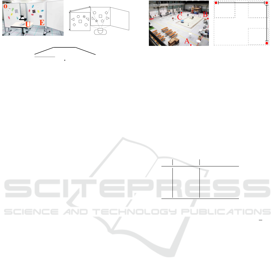
(a) Real situation.

(b) Schematic fronal view.

Figure 3: Small-scale setup: (U)ser, (E)nvironment, and

(O)ccluder.

tion error of MAE

Qualysis

(pos.)=1.2mm (min: 0.1mm;

max: 8.9mm; SD: 2.17mm) and a mean absolute

orientation error of MAE

Qualysis

(ori.)=0.52

◦

(min:

0.01

◦

; max: 1.7

◦

; SD: 0.76

◦

) to estimate 6DoF poses

on 45m×35m×7m=11.025m

The evaluator receives different data from the two

sides. The reference system sends the current UTC

timestamp and the absolute position and orientation at

300Hz on average (SD=0.01Hz). In addition, the ARs

send their state (reliability level from 0%=not work-

ing to 100%=working) and the number of features

(number of vertices of the current room mesh, i.e.,

the number of unique synthetic or natural features)

that yield the relative position and orientation (AR

avg. 31Hz, SD=3.6Hz; AR

: avg. 27Hz, SD=7.9Hz;

: avg. 60Hz, SD=11.2Hz). Note, that the coordi-

nate systems of the ARs are always relative to the ref-

erence system’s coordinate system. To align both, we

simply match the origins of the two coordinate sys-

tems and align the directions of the x- and y-axes.

The evaluator employs the cross-platform AR en-

gine Unity3D (version 2018 LTS). To synchronize the

data packets received from the two sides it uses both

the UTC timestamp of the common WiFi access point

and the frames per second rate (FPS). We also use

Unity3D to implement the visualization of the user

interface and to control the experiment, i.e., to start

and stop the recording of the data which we trigger

with a typical input device, see Fig. 2(d). For each

experiment, the evaluator also provides visual feed-

back on the successful calibration and alignment of

the reference and measurement setup.

The small-scale setup (Fig. 3) is a feature-rich en-

vironment consisting of 3 areas E

–E

(static boards

of size 2m×2m) that are positioned with an angle of

160

◦

between them. While E

and E

are feature-

free, the center board E

has a set of unique syn-

thetic features whose poses the reference system can

determine. There is also a moveable occluder board

O that we roll into the user’s ﬁeld of view (FoV) in

certain scenarios of the experiment. Board O has the

(a) Real situation.

30m

C B

(b) Schematic top-view.

Figure 4: Large-scale setup: Cubicles A–C.

same size but a different set of synthetic features. Ac-

cording to Dilek et al. (2018) we chose boards with

white backgrounds to avoid uncontrolled additional

features. The distance between U, O, and E is chosen

so that E and O completely ﬁll the user’s FoV.

Large-scale Setup. Fig. 4 shows the large-scale

setup that. On a ﬂoor of 30m×30m there are three

cubicles A–C and several natural features.

4.2 Study Design

Table 1: Small-scale scenes.

(U)ser (O)ccluder

static absent

dynamic absent

static dynamic

dynamic dynamic

dynamic* dynamic*

* synchronous movement of U and O,

with the same start- and end-points.

Small-scale Study. We studied ﬁve different Small-

scale motion scenarios S

–S

. In all of them the static

environment E

–E

remained the same. As Table 1

shows, in S

and S

there was no occluder. In the

other three scenarios O moved while the user either

remained static or moved as well. In S

the movement

of U and O was synchronous and the individual start-

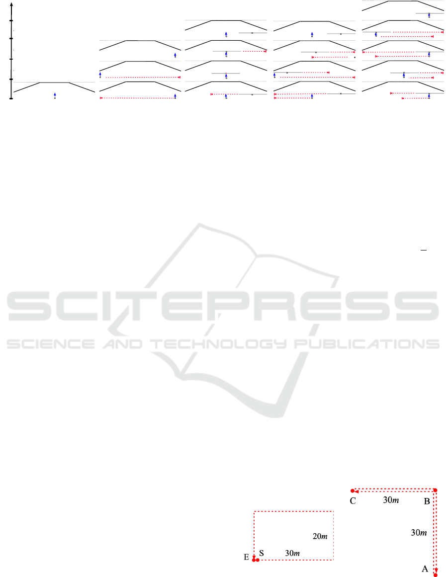
and end-points of both were the same. Fig. 5 shows

snapshots of the scene over time. The red dashed ar-

rows indicate the movement paths that will happen

before the next snapshot is taken.

We claim that these scenarios mimic what fre-

quently happens in industry settings when workers are

busy in a cubicle and they or their surrounding objects

may move within the cubicle.

Before we started recording the poses in each of

the ﬁve scenarios, we calibrated the AR platforms.

To do so, we aligned the relative coordinate system

of the AR systems with the absolute coordinate sys-

tem of the reference system on the basis of the ﬁrst

measured data points. This eliminates any differences

in position and orientation. Based on this initial ad-

justment, both systems then track the same current

pose within the experiment. After the calibration we

Localization Limitations of ARCore, ARKit, and Hololens in Dynamic Large-scale Industry Environments

311

time

t=2

t=1t=0

t=3 t=4

(a) S

: static U,no O.

(b) S

: dynamic U,

no O.

: static U,

dynamic O.

(d) S

: dynamic U

and dynamic O.

(e) S

: synchronous

dynamic* U and O.

Figure 5: Small-scale experiment: Exemplary snapshots for the scenarios S

to S

; (U)ser, (E)nvironment, and (O)ccluder;

red arrows indicate motion over time from the bottom- to the top-row; blue arrows indicate the user’s viewing direction; gray

dotted lines indicate a wall; duration between the three snapshots varies between the S

; *synchronous dynamic motion: both

U and O have the same speeds and directions with the same individual start- and end-points.

slightly moved the AR platform to identify features of

the central board E

and thus to initialize the tracking.

For each scenario, we recorded measurement data

ten times and only present the mean values below.

(static U, no O) covers the real-world situation

of a static user, standing still in a static environment.

There is no occluder. In this and all of the subsequent

small-scale scenarios the view of the user is always

focused on E during the measurement.

In scenario S

(dynamic U, no O) the user per-

forms a lateral movement from the right to the left

side and back, at 0.5m/s on average, SD=0.25m/s.

(static U , dynamic O) is a real-world situa-

tion of a static user standing still in a dynamic en-

vironment. The occluder O moves into the user’s

FoV from the right. Once it reaches the center it

fully occludes the features of E

, presenting its own

features to the user instead. O then changes its di-

rection and moves back to the right. We used two

different O-velocities: fast=0.8m/s, SD=0.2m/s and

slow=0.3m/s, SD=0.1m/s.

In S

(dynamic U and O) both the user and the

occluder move, but independently of each other. The

user performs a lateral movement from the center to

the left, changes his/her direction, and moves to the

right, changes his/her direction, and moves back to

the center, at 0.5m/s on average, SD=0.25m/s. At the

same time O moves from the right to the left, changes

its direction, and moves back. On its way the oc-

cluder O temporarily hides the features of E

twice

(and presents its own features instead). We used the

same two O-velocities as in S

In S

(synchronous dynamic U and O) again

both the user and the occluder move, but their

speeds and directions are synchronized (velocity

SD(U,O)=0.9m/s) so that the occluder O always

hides the features of E

and presents its own fea-

tures instead. Both the user and the occluder start

from the right, move to the center, change their

directions, and move to the right, change their direc-

tions, and move to the left, and turn back to the right.

uses the same O-velocities, but this time also for U.

Large-scale Study. We studied two different Large-

scale scenarios L

and L

. Fig. 6 shows the movement

paths of the user U. We claim that both scenarios are

typical for an industry context with natural features:

workers are likely to move between cubicles that are

distant to each other. Again, we initially calibrated the

AR platforms before we started to record the pose for

each of the two scenarios. We again recorded mea-

surement data ten times and only present the mean

values below.

In L

a user moves within a static environment

with natural features and follows a rectangular path of

2×20m+2×30m=100m. The user starts in S and stops

in E where we relocalize, i.e., recalibrate the system

to determine the scaling and mapping errors.

In L

a user also moves within a static environ-

ment with natural features. The user starts in cubicle

A, walks to B, and stops in C. Then, we relocalize and

determine the scaling and mapping errors before the

user walks back to A via B. The trajectory length is

4×30m=120m. When back in A, we again relocalize

(a) L

: From (S)tart to

(E)nd.

(b) L

: From cubicles A

via B to C, and back.

Figure 6: Large-scale experiment: L

and L

show user tra-

jectories (red dashed arrows); same cubicles as in Fig. 4.

GRAPP 2020 - 15th International Conference on Computer Graphics Theory and Applications

312

and determine the errors.

To gauge how errors accumulate after the ﬁrst 60m

in cubicle C, there is a second set of measurements

without the relocalization.

4.3 Metrics

Tracking Accuracy. We evaluate the accuracy by

means of the mean absolute error (MAE) and the

mean relative error (MRE). We measure both errors

in terms of position error [m] and orientation error [

◦

MAE =

∑

i=1

− m

, (1)

where r

is the value from the reference system and

is the value measured in the AR system. The MAE

uses the same scale as the data being measured. The

mean relative error (MRE) is the following average:

MRE =

∑

i=1

||r

i+1

− r

| −|m

i+1

− m

(2)

where r

i+1

is the current and r

is the previous refer-

ence. m

i+1

is the current and m

is the previous mea-

sure. The MRE also uses the same scale as the data

being measured. The MRE expresses the scaling er-

rors with multiple measures based on n samples, i.e.,

the difference between reference and measurement of

n accumulated samples.

Initialization Accuracy. For each AR system we

physically align the HMD’s (measurement) coordi-

nate system, i.e., the x-axis of the body frame, with

the reference system’s coordinate system, i.e., the x-

axis of the system marked on the ﬂoor. Note, the eval-

uator provides feedback on the successful calibration,

i.e., when the reference and measurement setup are

aligned. We then calculate the translational and an-

gular differences between the AR system and the ref-

erence system. We again measure initialization accu-

racy in terms of position error and orientation error.

Relocalization Accuracy. Similarly, we use the off-

set between the coordinate systems of the AR systems

and the reference system to determine the relocaliza-

tion accuracy (both position and orientation errors) af-

ter each of the scenarios S

–S

and L

–L

The reliability R

i, j

∈ [−1;1] of AR

with j ∈

A,G,M spans from system crash [−1;0] to fully func-

tional ]0;1] per frame i and is determined as:

i, j

f eat(AR

) − f ail

f eat

(AR

)

max

f eat

(AR

) − f ail

f eat

(AR

)

, (3)

with the number of currently available features

f eat(AR

) in a scene, the number of features

f ail

f eat

(AR

) that cause AR

to fail (AR

re-

quires at least f ail

f eat

(AR

)+1 to estimate a pose:

=15, AR

=26, AR

=63), and the maximal num-

ber max

f eat

(AR

) of features that we ever observed

for AR

being able to process in our experiments. It

is an engineering task to ﬁnd f ail

f eat

(AR

). Note that

f eat(AR

) ≤ f ail

f eat

(AR

) yields a system crash.

5 EVALUATION RESULTS

We present the measurements of the small- and the

large-scale experiment, before we discuss the results.

5.1 Small-scale Measurements

Because of space restrictions we cannot show a ﬁgure

per scenario, per occluder speed, and per AR system.

We thus only show numbers and curves for the ﬁve

scenarios S

–S

(slow speed only) that were measured

with AR

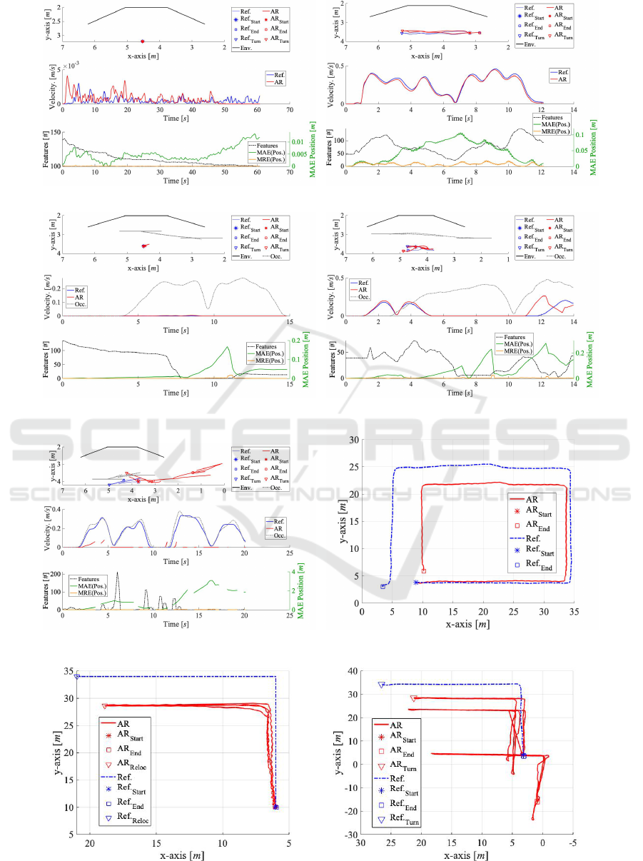
, see Figs. 7(a-e). Table 2 holds condensed

numbers for all cases. The general structure of the

ﬁve Figs. 7(a-e) is as follows: They have three graphs

each. The upper graph corresponds to the schematic

top-view known from Fig. 5. The static environment

and the occluder’s starting, turning, and ﬁnal posi-

tions (S

–S

) are shown in black. For the user tra-

jectories the upper graph shows the AR

measure-

ments (red) and the reference values (blue). Devia-

tions between the red and blue curves, i.e., absolute

pose errors, are easy to spot. The occluder’s trajec-

tory is shown in grey. The second of the three graphs

illustrates the motion velocities of the captured poses.

The bottom graph shows the number of features f eat

over time (black, dashed) and also the position errors

MAE (green) and MRE (orange).

Measurement Results That Can Be Generalized

across S

–S

. As the user’s focus was ﬁxed to the

environment in the small-scale experiment there were

no signiﬁcant orientation errors, see the orientation

columns in Table 2. All the initialization errors are

also unremarkable throughout S

–S

and all ARs. The

initialization errors are stable across S

–S

as we al-

ways moved the features in about the same way when

setting up. The relocalization errors show no signiﬁ-

cant changes across S

–S

and vary around 5cm. But

there is the trend that fast motion lowers and slow mo-

tion increases the relocalization errors.

The tracking accuracy is more interesting as the

position errors, the number of features, and the reli-

ability scores vary between the ARs and the scenar-

ios. Across S

–S

, AR

shows the smallest errors,

the highest number of features, and the best reliabil-

ity. AR

comes second. AR

suffers from the largest

errors, the lowest number of features, and the worst

reliability. The standard deviations (SD) support this:

Localization Limitations of ARCore, ARKit, and Hololens in Dynamic Large-scale Industry Environments

313

(a) S

(static U, no occluder). (b) S

(dynamic U, no occluder).

(static U, with a slow occluder). (d) S

(dynamic U, with a slow occluder).

(e) S

(dynamic U, synchronized with a slow occluder). (f) L

(rectangular trajectory, 100m).

(g) L

(cubicle walk, 120m, w. reloc. after 60m). (h) L

(cubicle walk, 120m, w/o intermediate reloc.).

Figure 7: AR

measurements; (a-e) for S

–S

: trajectories, velocities, features, and accuracy; (f-h) for L

–L

: trajectories.

GRAPP 2020 - 15th International Conference on Computer Graphics Theory and Applications

314

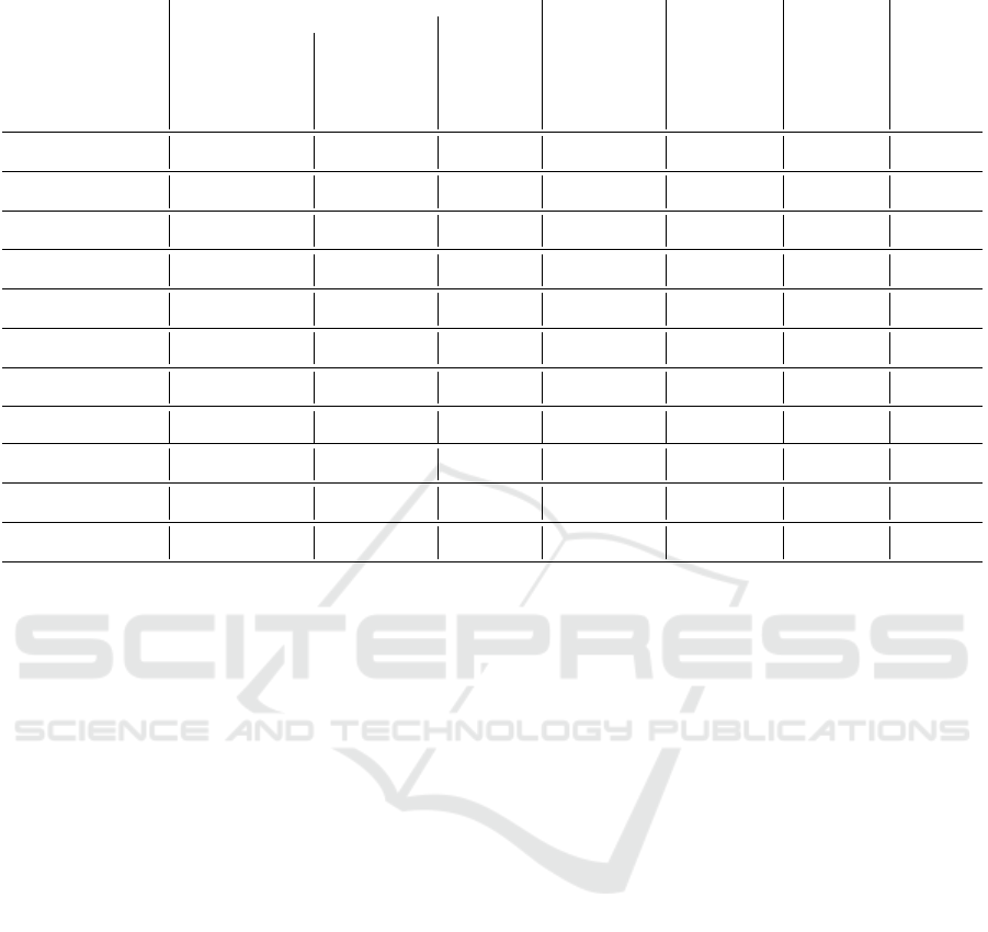
Table 2: Condensed measurements (best ones in bold).

Tracking Initialization Relocalization Features * Reliability *

Position Orientation

Scenario

MAE(AR

)[cm]

MAE(AR

)[cm]

MAE(AR

)[cm]

MRE(AR

)[cm]

MRE(AR

)[cm]

MRE(AR

)[cm]

MAE(AR

)[

◦

]

MAE(AR

)[

◦

]

MAE(AR

)[

◦

]

MAE(AR

)[cm]

MAE(AR

)[cm]

MAE(AR

)[cm]

MAE(AR

)[cm]

MAE(AR

)[cm]

MAE(AR

)[cm]

[#]

[%]

(static U , no O) 2.5 5.7 2.2 0.4 0.9 0.8 1.7 3.2 1.5 16.2 29.4 11.6 6.2 9.4 7.6 14 123 359 0 36 59

SD 2.1 2.7 1.2 0.02 0.07 0.01 0.8 2.3 0.6 7.3 11.9 5.6 2.3 4.9 1.6 1 13 57 0 0 0

(dyn. U, no O) 8.1 12.3 7.4 2.1 3.7 0.7 2.3 1.5 0.9 16.2 21.3 9.8 5.9 7.1 4.7 46 183 391 24 58 65

SD 2.2 2.8 1.9 0.9 1.3 0.8 4.1 3.8 1.7 5.9 17.1 4.9 1.7 5.3 3.2 61 137 298 35 41 43

3,slow

(static U , dyn. O) 17.2 19.3 13.1 4.9 5.2 4.6 2.4 4.5 2.1 18.1 29.3 8.9 9.3 19.7 6.8 18 46 143 3 7 16

SD 2.5 3.8 2.5 1.6 1.7 1.3 3.5 4.5 2.9 4.5 11.4 3.8 2.1 4.9 4.1 53 87 125 29 23 12

3, f ast

(static U , dyn. O) 16.3 17.1 11.0 3.9 4.1 3.4 2.4 4.5 2.1 17.9 28.1 8.7 8.2 17.3 5.5 24 61 213 7 13 30

SD 2.4 3.6 1.9 1.9 2.1 1.8 4.4 4.7 2.8 5.4 10.1 4.1 1.9 4.1 1.3 45 77 121 23 19 12

4,slow

(dyn. U & O) 18.1 21.2 17.8 2.4 3.5 0.9 3.7 3.9 2.5 17.2 18.3 16.8 7.9 6.8 5.2 37 103 331 17 29 53

SD 4.1 4.5 3.3 1.5 2.7 1.3 3.4 5.1 2.4 9.1 9.4 5.8 2.1 3.8 5.2 68 188 206 41 60 28

4, f ast

(dyn. U & O) 16.2 19.5 14.1 1.6 2.7 0.8 4.9 5.8 3.1 16.8 17.3 15.7 6.7 8.8 4.3 73 208 421 44 67 71

SD 4.1 4.5 3.3 1.5 2.7 1.3 3.4 5.1 2.4 5.8 9.4 9.1 2.1 3.8 5.2 57 166 187 32 52 25

5,slow

(sync. dyn. U & O) 87.3 112.9 76.3 21.8 26.4 19.1 3.9 4.3 2.4 15.7 16.8 14.9 7.3 9.8 6.4 21 37 88 5 4 5

SD 69.3 82.1 50.6 11.9 14.3 7.7 3.4 4.1 3.7 5.2 4.7 8.2 1.3 2.6 1.1 88 247 366 56 82 60

5, f ast

(sync. dyn. U & O) 85.1 108.3 73.2 19.7 23.8 17.3 4.6 6.1 4.0 14.9 15.9 12.8 6.5 10.7 5.9 27 54 117 10 11 11

SD 61.4 78.3 47.4 13.7 16.3 6.6 3.1 5.7 2.9 5.3 6.4 4.9 3.5 4.3 1.2 76 201 315 46 65 50

(static U , no O) - - 601.2 - - 0.7 - - 3.5 - - 32.8 - - 41.5 - - 487 - - 84

SD - - 24.3 - - 2.3 - - 1.6 - - 5.7 - - 4.3 - - 42 - - 0

(static U , no O) - - 437.9 - - 0.9 - - 4.1 - - 29.9 - - 36.2 - - 477 - - 82

SD - - 33.9 - - 1.9 - - 4.2 - - 6.3 - - 5.7 - - 56 - - 0

2,w/o

relocalization

- - 1728.5 - - 0.6 - - 3.8 - - 28.3 - - - - - 491 - - 85

SD - - 43.6 - - 4.1 - - 1.2 - - 5.7 - - - - - 66 - - 0

* Feature counts ([min.;max.]) for all scenarios: f eat(AR

) ∈ [14; 147], f eat(AR

) ∈ [25; 296], and f eat(AR

) ∈ [62; 567].

there is lower variance for AR

(within and across all

measures) than for AR

. AR

has the highest SD.

Now that we have sketched the big picture, let us

discuss the scenarios individually.

Measurement Results That Are Speciﬁc for S

–S

and S

yield the lowest absolute and relative posi-

tion errors and orientation errors in all measures for

all ARs. While S

yields the lowest MAE of the po-

sition (2.2cm) and orientation (0.9

◦

), S

provides the

lowest MRE of the position (0.3cm) across all exper-

iments. In Figs. 7(a+b) we observe that when there

is no velocity in S

the number of features remains

stable. With dynamics in S

there is also a varying

number of features. The reliability scores in Table 2

support these ﬁndings as there are higher scores when

the user moves faster (or moves at all).

Compared to S

–S

, there are higher absolute and

relative position errors and orientation errors in S

and S

, see Table 2. As before, a moving user

yields higher absolute position errors (MAE>10cm)

but lower relative errors (MRE<1cm), even if there

is an occluder. This also holds for the two fast mo-

tion variants. Figs. 7(c+d) again show that a more

dynamic user sees more features, which then results

in a higher reliability score. In S

the movement of

the occluder has a dramatic impact on the number of

features and the reliability scores: both drop to lower

values once the occluder hides E

, and they remain

on that level when the occluder leaves the user’s FoV

again. We discuss this in detail in Sec. 6.

yields the highest position and orientation er-

rors of all measurements with all ARs. This time the

absolute position error is more than 5 times higher

for all ARs. Also the number of features and the re-

liabilities are the lowest among all experiments. The

user moves synchronously at the same speed in the

same direction as the occluder. For the user, the oc-

cluder’s features do not move, as they move quasi par-

allel to his/her FoV, see the red curve in the velocity

graph of Fig. 7(e). Hence, the ARs cannot distinguish

between their self-motion and the motion of the oc-

cluder’s features. In total, the ARs interpret this as if

there is no movement at all. Because even in these sit-

uations, they apparently do not use inertial sensors to

sense motion and continue to rely solely on the cam-

era’s motion estimates. However, due to the study de-

sign there may be moments when the ARs still occa-

sionally ﬁnd features to stabilize their internal feature

tracking state.

5.2 Large-scale Measurements

For our large-scale experiments we can only show the

measurements of AR

because both AR

and AR

were unable to initialize and localize. The bottom

rows of Table 2 and Figs. 7(f-h) hold the data. The

graph layouts correspond to the schematic top-view

known from Fig. 6. For the user trajectories they show

Localization Limitations of ARCore, ARKit, and Hololens in Dynamic Large-scale Industry Environments

315

Table 3: Average scaling error in the large-scale scenarios.

Distance, SD, td [m] Scaling Error, SD

100, 9, 101.2 5.94cm/m, 0.21cm

60, 3, 62.8 6.97cm/m, 0.19cm

2,w/o

120, 12, 118.76 14.55cm/m, 2.83cm

both the AR measurements (red) and the reference val-

ues (blue). Again, deviations, i.e., absolute pose er-

rors, are easy to spot.

Measurement Results That Can Be Generalized

across L

–L

. As before, the orientation, initializa-

tion, and relocalization errors are unremarkable, see

Table 2. However, because of the much larger dis-

tances both the initialization and relocalization errors

are higher than for S

–S

, but they show similar vari-

ances. The number of features is higher for L

–L

(at

lower variance) than for S

–S

and results in the high-

est reliability values across all experiments.

Table 2 shows that the absolute position errors

grow with the length of the trajectory that is traveled

without relocalization (60m in L

, 100m in L

, and

120m in L

). This can also be seen in Figs. 7(f-h).

When you follow the trajectory of the user along the

space, the distances between the red and blue curves

grow. When there is no intermediate relocalization,

the effect is much stronger than in plain L

. After

each measurement or in the intermediate relocaliza-

tion phase we calculated the scaling error S=

MAE

position

where td is the traveled distance, see Table 3. Note,

that the distance and td differ because of the SD.

Whereas the scaling error is about the same

for L

and L

with a relocalization after 60m,

(6.65cm/m (=5.94+6.97/2) on average), it ”explodes”

(14.4cm/m) in L

when no relocalization is done for

about 120m. We discuss this in detail below.

6 DISCUSSION

The occluder-free scenarios S

and S

yield the lowest

absolute position error for all ARs. This is because the

SLAM techniques are able to separate a user’s self-

motion from the static environment. In contrast, the

techniques struggle to accurately tell self-motion and

feature motion (of the occluder) apart. This is sup-

ported by the scenarios S

–S

that yield higher abso-

lute errors when an occluder is present and when the

occluder hides the features of the environment longer

or more often.

Velocity has an impact. Although, a higher ve-

locity leads to blurry camera images and hence fewer

features, our motion scenarios resulted in more fea-

tures and a better relative position accuracy. We think

that faster movement reduces the duration of situa-

tions where there is an occluder in the FoV of the user,

and therefore the duration of a disturbance is shorter,

which leads to smaller accumulated errors.

We suppose that SLAM implementations make

use of an internal ﬁlter that estimates the position in

case of a noisy input (a varying number of features

or unknown features), i.e., when there are dynamics

of either U or O or both. After a while, the AR sys-

tems stabilize the ﬁlter with ground truth knowledge

(known features) and relocalize. What supports this

assumption is the slight delay and offset that exist be-

tween the number of features and the position errors

in the graphs in Figs. 7(d) (compare the ”Features”

and the ”MAE” curves within the [4.5s;6s] interval in

the bottom graph).

In all our scenarios there is an inverse correlation

between a high reliability score (number of features)

and a low MRE of the position (and vice versa). There

is no such inverse correlation with the MAE. On the

contrary, especially in the L

scenarios when the R

is high, the MRE is low, but the MAE is also high.

We suppose that the initialization and relocalization

errors have a stronger impact on the MAE than the

number of features. This is in line with ﬁndings by

(Marchand et al., 2016; Terashima and Hasegawa,

2017) as VISLAM for the ARs works like a pedestrian

dead reckoning (PDR) algorithm. Here, the initial-

ization and relocalization errors stabilize the absolute

position while the relative position updates (estimated

based on the features) accumulate small errors (with

more features) over time (scaling error).

The impact of the scaling errors (accumulation of

small relative position errors) depends on the scale.

There is little impact in the small-scale scenarios, but

the AR measurements and the reference positions dif-

fer a lot in the large-scale scenarios. This indicates

that the AR systems exploit both the initialization

and relocalization to stabilize the absolute positions.

However, when they internally are conﬁdent about the

input (no varying or unknown features) they rely on

the relative position estimates. Hence, for SLAM to

perform best, both MAE and MRE must be reduced.

We think that the reason for AR

performing sig-

niﬁcantly better (in all measures, in all scenarios) than

or AR

is that AR

exploits a special RGB − D

sensors, while the other only use a single RGB sen-

sor. As there is no such hardware difference between

and AR

a potential explanation why AR

out-

performs AR

may be that its SLAM is better opti-

mized for its sensors.

In scenarios with relocalization and high reliabil-

ity the ARs achieve a low MRE but a high MAE of the

position. But with a long trajectory even a small rel-

ative error accumulates and grows into a signiﬁcant

GRAPP 2020 - 15th International Conference on Computer Graphics Theory and Applications

316

relative drift and absolute offset. In the large-scale

scenarios the absolute error lineraly increases as there

is an average scaling error of approximately 5.9cm/m

if there are intermediate relocalizations after at most

100m. However, we postulate that this linearity only

holds when there are no changes or only slight rota-

tions of up to 90

◦

in the movement direction. The

counterexample (S=14.5cm/m) is L

without relocal-

ization and with its abrupt 180

◦

rotation.

The general applicability of the reliability score R

(soley based on features) cannot be guaranteed, as we

saw that there are situations when a higher R does not

correlate with the MAE but with the MRE of the po-

sition. Because a single metric as the MRE, is not

enough to evaluate and validate accuracy and reliabil-

ity of ARs our R could be improved.

Although there are many other AR platforms to-

day, e.g., Wikitude (Fraga-Lamas et al., 2018), we

chose AR

, AR

, and AR

because they are mar-

ketable, inexpensive, pre-installed, and widely used

by our industrial customers. We focused on these

three commercial systems as these are well estab-

lished in both the consumer and industrial markets

and therefore their manufacturers offer customer sup-

port. Industrial customers are unwilling to work with

research and development versions of AR systems

just because they provide more accurate positions in

some special cases.

7 CONCLUSION

We studied the applicability of today’s popular AR

systems (Apple ARKit, Google ARCore, and Mi-

crosoft Hololens) in industrial contexts (large area of

1,600m

, walking distances of up to 120m between

cubicles, and dynamic environments with volatile nat-

ural features). The Hololens with its special RGB-D

sensors outperformed ARKit (RGB only) in all exper-

iments. ARCore showed the worst results.

In a nutshell, we found that standing still does

not result in any features while motion enables the

detection of features. However, abrupt movement

changes at high speeds reduce the number of de-

tectable features. A low/high number of features

yields a low/high reliability. And a low/high reliabil-

ity results in high/low relative and absolute position

errors. Low/high position errors enable/disable AR

systems in large scale industry environments.

Regardless of the AR systems, we only found good

position accuracies in static environments and when

only the user moves. Having more identiﬁable fea-

tures helps. Whereas movement results in detectable

features and hence in reliabilities and relative position

accuracies, on longer trajectories and at higher veloc-

ities there is still a signiﬁcant amount of accumulated

drift. Hence, AR systems are applicable in industry

settings when a worker’s surroundings are static and

when process streets between cubicles are short and

only require smooth directional changes.

When relocalization is possible within at least

100m of the trajectory, the AR systems accumulate a

linear scaling error of 6.65cm/m, on average. When

there is no intermediate relocalization available, the

best system only yields a MAE of 17.28m per 120m,

with a scaling error of up to 14.4cm/m, which is

clearly too much for industry-strength applications.

We identiﬁed two typical industry scenarios that

revealed problems of the AR systems: (a) They tend

to crash when a user moves while a surrounding ob-

ject, e.g., a fork lift, synchronously moves on the side.

(b) There are system instabilities when workers ran-

domly enter or leave the ﬁeld of view of the AR sys-

tem and temporarily occlude known features (as the

systems can hardly distinguish between self-motion

and feature motion).

ACKNOWLEDGMENTS

This work was supported by the Bavarian Min-

istry for Economic Affairs, Infrastructure, Trans-

port and Technology through the Center for Ana-

lytics—Data—Applications (ADA-Center) within the

framework of “BAYERN DIGITAL II”.

REFERENCES

Burri, M., Nikolic, J., Gohl, P., Schneider, T., Rehder, J.,

Omari, S., Achtelik, M. W., and Siegwart, R. (2016).

The EuRoC micro aerial vehicle datasets. Intl. J. of

Robotics Research, 35(10):1157–1163.

Choset, H. M., Hutchinson, S., Lynch, K. M., Kantor,

G., Burgard, W., Kavraki, L. E., and Thrun, S.

(2005). Principles of robot motion: theory, algo-

rithms, and implementation. Intelligent Robotics and

Autonomous Agents. MIT Press, Cambridge, USA.

Cort

es, S., Solin, A., Rahtu, E., and Kannala, J. (2018). AD-

VIO: An authentic dataset for visual-inertial odom-

etry. In Proc. European Conf. Computer Vision

(ECCV), pages 419–434, Munich, Germany.

Dilek, U. and Erol, M. (2018). Detecting position us-

ing ARKit II: generating position-time graphs in real-

time and further information on limitations of ARKit.

Physics Education, 53(3):5–20.

Durrant-Whyte, H. and Bailey, T. (2006). Simultaneous lo-

calization and mapping: part I. Robotics & Automa-

tion Magazine, 13(2):99–110.

Localization Limitations of ARCore, ARKit, and Hololens in Dynamic Large-scale Industry Environments

317

Feigl, T., Mutschler, C., and Philippsen, M. (2018). Super-

vised learning for yaw orientation estimation. In Proc.

Intl. Conf. Indoor Navigation and Positioning (IPIN),

pages 103–113, Nantes, France.

Fraga-Lamas, P., Fern

andez-Caram

es, T. M., Blanco-

Novoa,

O., and Vilar-Montesinos, M. A. (2018). A

review on industrial augmented reality systems for the

industry 4.0 shipyard. In Proc. Intl. Conf. Intelligent

Robots and Systems (IROS), pages 131–139, Madrid,

Spain.

Geiger, A., Lenz, P., Stiller, C., and Urtasun, R. (2013).

Vision meets robotics: The KITTI dataset. Intl. J. of

Robotics Research, 18(17):6908–6926.

Handa, A., Whelan, T., McDonald, J., and Davison, A. J.

(2014). A benchmark for RGB-D visual odometry,

3D reconstruction and SLAM. In Proc. Intl. Conf.

Robotics and Automation (ICRA), pages 1524–1531,

Hong Kong, China.

Kasyanov, A., Engelmann, F., St

uckler, J., and Leibe, B.

(2017). Keyframe-based visual-inertial online SLAM

with relocalization. In Proc. Intl. Conf. Intelligent

Robots and Systems (IROS), pages 6662–6669, Van-

couver, Canada.

Kato, H. and Billinghurst, M. (1999). Marker tracking and

HMD calibration for a video-based augmented reality

conferencing system. In Proc. Intl. Workshop on Aug-

mented Reality (IWAR), pages 85–94, San Francisco,

CA.

Kerl, C., Sturm, J., and Cremers, D. (2013). Dense visual

SLAM for RGB-D cameras. In Proc. Intl. Conf. Intel-

ligent Robots and Systems (IROS), pages 2100–2106,

Tokyo, Japan.

Klein, G. and Murray, D. (2007). Parallel tracking and

mapping for small AR workspaces. In Proc. Intl.

Workshop on Augmented Reality (ISMAR), pages 1–

10, Nara, Japan.

ofﬂer, C., Riechel, S., Fischer, J., and Mutschler, C.

(2018). Evaluation criteria for inside-out indoor po-

sitioning systems based on machine learning. In Proc.

Intl. Conf. Indoor Positioning and Indoor Navigation

(IPIN), pages 1–8, Nantes, France.

Li, P., Qin, T., Hu, B., Zhu, F., and Shen, S. (2017).

Monocular visual-inertial state estimation for mobile

augmented reality. In Proc. Intl. Conf. Intelligent

Robots and Systems (IROS), pages 11–21, Vancouver,

Canada.

Li, W., Saeedi, S., McCormac, J., Clark, R., Tzoumanikas,

D., Ye, Q., Huang, Y., Tang, R., and Leuteneg-

ger, S. (2018). Interiornet: Mega-scale multi-sensor

photo-realistic indoor scenes dataset. arXiv preprint

arXiv:1809.00716, 18(17).

Linowes, J. and Babilinski, K. (2017). Augmented Real-

ity for Developers: Build practical augmented reality

applications with Unity, ARCore, ARKit, and Vuforia.

Packt Publishing Ltd, Birmingham, UK.

Liu, H., Chen, M., Zhang, G., Bao, H., and Bao, Y.

(2018). Ice-ba: Incremental, consistent and efﬁcient

bundle adjustment for visual-inertial SLAM. In Proc.

Intl. Conf. Computer Vision and Pattern Recognition

(CVPR), pages 1974–1982, Salt Lake City, UT.

Marchand, E., Uchiyama, H., and Spindler, F. (2016). Pose

estimation for augmented reality: A hands-on sur-

vey. Trans. Visualization and Computer Graphics,

22(12):2633–2651.

Marques, B., Carvalho, R., Dias, P., Oliveira, M., Fer-

reira, C., and Santos, B. S. (2018). Evaluating and

enhancing Google Tango localization in indoor en-

vironments using ﬁducial markers. In Proc. Intl.

Conf. Autonomous Robot Systems and Competitions

(ICARSC), pages 142–147, Torres Vedras, Portugal.

Mur-Artal, R. and Tardos, J. D. (2017). ORB-SLAM2: An

open-source SLAM system for monocular, stereo, and

RGB-D cameras. Trans. Robotics, 33(5):1255–1262.

Neumann, U. and You, S. (1999). Natural feature tracking

for augmented reality. Trans. on Multimedia, 1(1):12–

20.

Palmarini, R., Erkoyuncu, J. A., and Roy, R. (2017). An

innovative process to select augmented reality (AR)

technology for maintenance. In Proc. Intl. Conf. Man-

ufacturing Systems (CIRP), pages 23–28, Taichung,

Taiwan.

Regenbrecht, H., Meng, K., Reepen, A., Beck, S., and Lan-

glotz, T. (2017). Mixed voxel reality: Presence and

embodiment in low ﬁdelity, visually coherent, mixed

reality environments. In Proc. Intl. Conf. Intelligent

Robots and Systems (IROS), pages 90–99, Vancouver,

Canada.

Saputra, M. R. U., Markham, A., and Trigoni, N. (2018).

Visual SLAM and structure from motion in dynamic

environments: A survey. Comput. Surv., 51(2):1–36.

Schubert, D., Goll, T., Demmel, N., Usenko, V., St

ockler,

J., and Cremers, D. (2018). The TUM VI benchmark

for evaluating visual-inertial odometry. In Proc. Intl.

Conf. Intelligent Robots and Systems (IROS), pages

6908–6926, Madrid, Spain.

Simon, G., Fitzgibbon, A., and Zisserman, A. (2000).

Markerless tracking using planar structures in the

scene. In Proc. Intl. Workshop Augmented Reality (IS-

MAR), pages 120–128, Munich, Germany.

Taketomi, T., Uchiyama, H., and Ikeda, S. (2017). Vi-

sual SLAM algorithms: a survey from 2010 to 2016.

Trans. Computer Vision and Applications, 9(1):452–

461.

Terashima, T. and Hasegawa, O. (2017). A visual-SLAM

for ﬁrst person vision and mobile robots. In Proc. Intl.

Conf. Intelligent Robots and Systems (IROS), pages

73–76, Vancouver, Canada.

Vassallo, R., Rankin, A., Chen, E. C. S., and Peters, T. M.

(2017). Hologram stability evaluation for Microsoft

Hololens. In Proc. Intl. Conf. Robotics and Automa-

tion (ICRA), pages 3–14, Marina Bay Sands, Singa-

pore.

Voinea, G.-D., Girbacia, F., Postelnicu, C. C., and Marto, A.

(2018). Exploring cultural heritage using augmented

reality through Google’s Project Tango and ARCore.

In Proc. Intl. Conf. VR Techn. in Cultural Heritage,

pages 93–106, Brasov, Romania.

Yan, D. and Hu, H. (2017). Application of augmented real-

ity and robotic technology in broadcasting: A survey.

Intl. J. on Robotics, 6(3):18–27.

GRAPP 2020 - 15th International Conference on Computer Graphics Theory and Applications

318