Detection and Categorisation of Multilevel High-sensitivity

Cardiovascular Biomarkers from Lateral Flow Immunoassay Images via

Recurrent Neural Networks

Min Jing

, Donal McLaughlin

, David Steele

, Sara McNamee

, Brian MacNamee

, Patrick Cullen

Dewar Finlay

and James McLaughlin

Nanotechnology and Integrated BioEngineering Centre (NIBEC), Ulster University, U.K.

Department of Physics, University College London, U.K.

Biocolor Ltd, U.K.

School of Computer Science, University College Dublin, Republic of Ireland

Keywords:

Lateral Flow Immunoassays (LFA) Image, High-sensitivity Cardiovascular Biomarkers, Classiﬁcation, Long

Short-Term Memory (LSTM), Point-of-Care (PoC).

Abstract:

Lateral Flow Immunoassays (LFA) have the potential to provide low cost, rapid and highly efﬁcacious Point-

of-Care (PoC) diagnostic testing in resource limited settings. Traditional LFA testing is semi-quantitative

based on the calibration curve, which faces challenges in the detection of multilevel high-sensitivity biomark-

ers due its low sensitivity. This paper proposes a novel framework in which the LFA images are acquired

from a designed CMOS reader system under controlled lighting. Unlike most existing approaches based on

image intensity, the proposed system does not require detection of region of interest (ROI), instead each row

of the LFA image was considered as time series signals. The Long Short-Term Memory (LSTM) network was

deployed to classify the LFA data obtained from cardiovascular biomarker, C-Reactive Protein (CRP), at eight

concentration levels (within the range 0-5mg/L) that are aligned with clinically actionable categories. The per-

formance under different arrangements for input dimension and parameters were evaluated. The preliminary

results show that the proposed LSTM outperforms other popular classiﬁcation methods, which demonstrate

the capability of the proposed system to detect high-sensitivity CRP and suggests the potential of applications

for early risk assessment of cardiovascular diseases (CVD).

1 INTRODUCTION

Cardiovascular disease (CVD) is considered as a ma-

jor threat to global health. There is a growing demand

for a range of portable, rapid and low cost biosens-

ing devices for the early detection of CVD. Lateral

Flow Immunoassays (LFA) are effective Point-of-

Care (PoC) devices that have attracted increased at-

tention recently because they can provide low cost,

rapid and highly efﬁcacious PoC diagnostic testing

in resource limited settings. Although LFA have

found widespread applications in POC diagnostics,

the low sensitivity of LFA limits their ability to de-

tect biomarkers, such as C-Reactive Protein (CRP),

which are normally present in low concentration in

blood (Ridker, 2003). CRP is a protein that increases

in the blood with inﬂammation or infection as well as

following a heart attack, surgery, or trauma. Accord-

ing to the National Institute of Health and Care Ex-

cellence’s (NICE) guidelines measuring CRP quanti-

tatively over concentration levels between 10mg/L to

100 mg/L can assess the severity of bacterial infec-

tion. High-sensitivity CRP (hs-CRP) tests performed

over a lower range (from 0.5mg/L to 10 mg/L) can be

used for early risk assessment of cardiovascular dis-

eases (CVD) (Ridker et al., 2000).

Detection of multilevel high sensitivity biomark-

ers via LFA testing is a challenging task. Studies have

been carried out to improve the detection sensitivity to

allow the development of high sensitivity assays (Tor-

res and Ridker, 2003), improve the labeling strate-

gies, enhance the optical and electrochemical trans-

ducers and explore the evolution of recognition (Mak

et al., 2016). Several methods have been developed to

enhance the sensitivity of LFA, such as sample con-

centration (Moghadam et al., 2015), ﬂuidic control

(Rivas et al., 2014), temperature–humidity technique

(Choi et al., 2016), probe-based signal enhancement

(Hu et al., 2013), enzyme-based signal ampliﬁcation

(Hu et al., 2014) and electrochemical devices-based

enhancement (Cheung et al., 2015). However, these

approaches require either external equipment, high-

Jing, M., McLaughlin, D., Steele, D., McNamee, S., MacNamee, B., Cullen, P., Finlay, D. and McLaughlin, J.

Detection and Categorisation of Multilevel High-sensitivity Cardiovascular Biomarkers from Lateral Flow Immunoassay Images via Recurrent Neural Networks.

DOI: 10.5220/0009117901770183

In Proceedings of the 13th International Joint Conference on Biomedical Engineering Systems and Technologies (BIOSTEC 2020) - Volume 2: BIOIMAGING, pages 177-183

ISBN: 978-989-758-398-8; ISSN: 2184-4305

177

cost reagents, or complicated fabrication with multi-

step procedure. To date, a low-cost, convenient and

equipment-free sensitivity enhancement method has

not been fully explored.

The use of smartphones has been reported for LFA

tests recently (Eltzov et al., 2015) (Quesada-Gonz

alez

and Merkoc¸i, 2017). However most of these applica-

tions are focused on simple binary classiﬁcation based

on image intensity. In most cases, the LFA image

data are obtained from scanners or smartphone cam-

eras, in which the performance can be affected by im-

age quality due to data being acquired under ambi-

ent lights. Most smartphone-based LFA testing are

based on popular machine learning approaches such

as Support Vector Machine (SVM). Very limited stud-

ies have attempted to apply neural networks to LFA

scenarios with a different focus to this study. For ex-

ample, Deep Belief Networks (DBN) were applied in

(Zeng et al., 2016) to improve the efﬁciency of ROI

detection rather than classiﬁcation. Multi-Layer Per-

ceptron (MLP) neural network was used in (Carrio

et al., 2015) for drugs-of-abuse detection based on av-

erage image intensity from the ROI, which assessed

saliva content but not blood based biomarkers.

Recurrent Neural Networks (RNN) are a class

of artiﬁcial neural networks that are capable of ex-

hibiting dynamic behaviour along a temporal se-

quence. Long Short-Term Memory (LSTM) networks

(Hochreiter and Schmidhuber, 1997) are a special

kind of RNN that are able to learn long-term depen-

dencies in time series data that have been success-

fully applied to speech recognition (Fern

andez et al.,

2007), language modelling (Jozefowicz et al., 2016)

and ECG arrhythmia detection (Picon et al., 2019)

(Xiong et al., 2018). In this study, we explore the po-

tential of applying LSTM to detect multilevel hs-CRP

by considering the LFA image data as time series sig-

nals.

Most existing approaches are based on the average

of image intensity from the LFA test line area, there-

fore the performance can be affected by the detection

of ROI. This study treats the LFA data along the sam-

ple ﬂow direction as time series signals therefore no

ROI detection is needed. Note that the purpose of this

study is not to analyse the LFA strip at discrete or

continuous time points as the assay proceeds. Instead

the LFA images were captured at a ﬁxed time point

(also known as an endpoint assay), following ‘com-

pletion’ of the lateral ﬂow assay. The LFA image is a

ﬁnal snapshot of the assay which contains a particular

spatial phenomenon, i.e., the leading edge is stronger

than the trailing edge, which also contains valuable

time-dependent information. Considering the LFA

as time series signals provides a novel perspective to

analyse the LFA data and helps to explore richer infor-

mation than image intensity. This study investigated

the dependence of data length, input dimension and

hidden layers in LSTM and the results demonstrate

the advantages and potential of the proposed frame-

work.

The rest of paper is organised as follows. In Sec-

tion 2 the structure of LFA is explained and an ex-

ample of LFA data is presented. In Section 3, the

proposed framework is described before the LSTM

network is explained, followed by the arrangement of

LFA data for the input sequence. The experimental

results are given in Section 4 with the conclusion and

future work presented subsequently.

2 LFA & IMAGE DATA

A schematic illustration of LFA is given in Figure

1, which shows the sample pad, sample ﬂow direc-

tion, conjugate pad, test line (T-line), control line (C-

line) and absorbent pad. The conjugate pad, usually

colloidal gold, is labelled with antibodies speciﬁc to

the target analyte. When the sample is placed on the

sample pad, it ﬂows by capillary action to the conju-

gate pad where the target analyte can interact (bind)

with these labelled conjugate antibodies. Conjugate

and any conjugate-sample complexes then travel lat-

erally along the strip. Upon reaching the T-line, any

formed conjugate-sample complexes are captured and

may begin to accumulate over the remainder of the

assay time. Once these reach sufﬁcient density a vi-

sual change occurs on the T-line. The C-line captures

any particle so therefore always appears regardless of

presence of the target analyte.

Figure 1: The schematic illustration of the LFA structure.

For traditional devices like an image scanner and

smartphone cameras, the image quality can be af-

fected by lighting conditions. In this study a CMOS

reader system has been designed in which the LFA

image data were acquired from an opaque box under

controlled lighting condition. Figure 2 gives exam-

ples of LFA strip images obtained at eight hs-CRP

concentration levels using the designed CMOS reader

system. The eight levels (in mg/L) are: 0, 0.05, 0.1,

0.2, 0.5, 1, 2.5 and 5. It can be seen that each strip

contains the C-line and T-line, in which the intensity

of the T-line changes according to the concentration

BIOIMAGING 2020 - 7th International Conference on Bioimaging

178

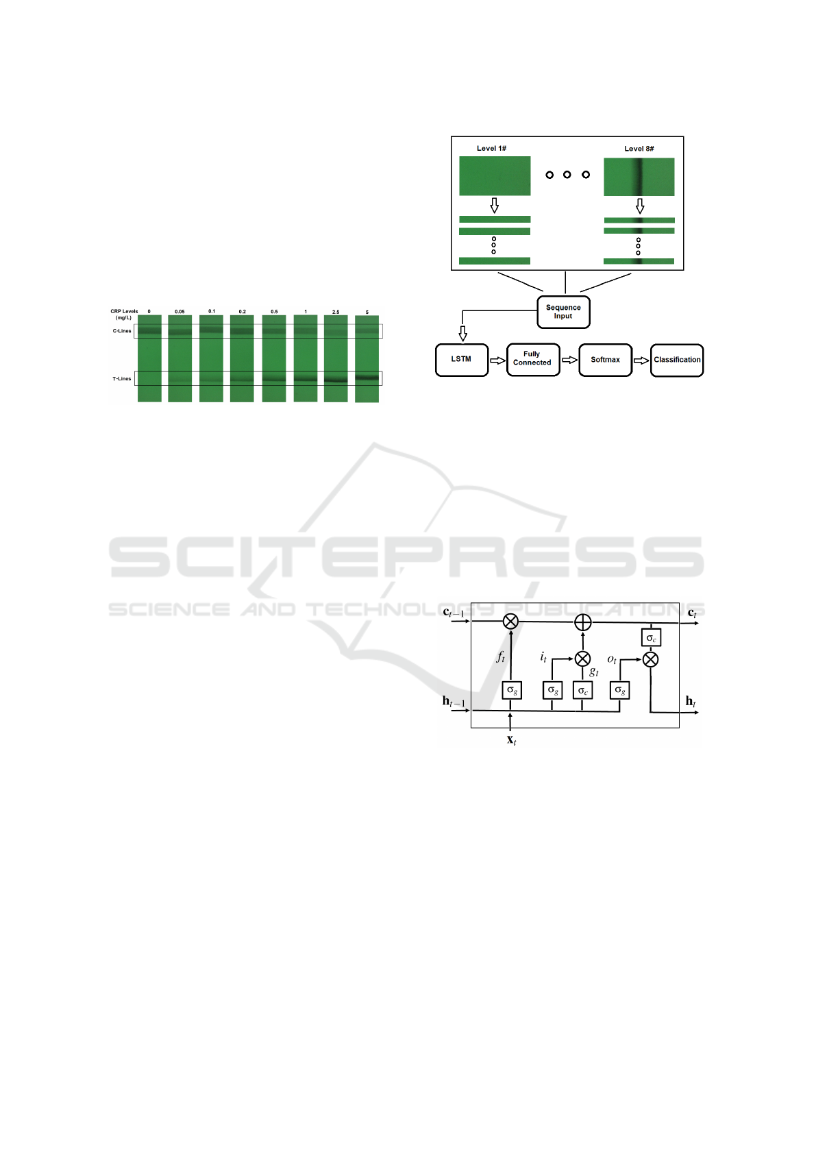
levels. It is also noticed that the position of the T-

line varies in each image. For those approaches based

on image intensity from the T-line area, the perfor-

mance is highly dependent on the accurate detection

of the T-line area. Features based on image intensity

works for simple binary classiﬁcation but a more so-

phisticated approach is needed for detection of high

sensitivity biomarkers, such as hs-CRP with a con-

centration level range lower than 5mg/L as outlined

in this study.

Figure 2: Examples of LFA strip images obtained from

eight hs-CRP concentration levels.

3 PROPOSED METHODS

3.1 System Overview

The proposed framework is shown in a block diagram

in Figure 3. For the purposes of this study, only the

area containing the T-line is needed for testing be-

cause the C-line does not reﬂect the change of con-

centration level in the sample. In a fully integrated

analysis system the formation of the C-line would be

used as a quality control check to ensure the assay

has performed correctly. Therefore, we directly select

the half LFA image containing the T-line without fur-

ther detection of T-line area. The half LFA image is

then divided into a number of mini LFA strips, which

are then used as the input sequences for the LSTM

network. The total number of input sequences is de-

pendent on the dimension of the mini strips. Once the

data has been arranged, they are fed into an LSTM

layer followed by a fully connected layer, a softmax

layer and an output layer for sequence classiﬁcation.

3.2 Long Short-Term Memory Network

LSTM is one type of RNN that can learn and remem-

ber over long sequences of input data, such as data

up to 200 to 400 time steps. Like most neural net-

works, one beneﬁt of LSTM is that it can learn from

the raw time series data directly and therefore does

not require feature extraction. In the LSTM, the sys-

tem updates the information for current state based on

the previous state via different gates. A block diagram

Figure 3: The block diagram for the proposed framework

including arrangement of LFA data for LSTM.

of the LSTM is given in Figure 4, which includes the

cell state c

and the hidden state (output state) h

time t. At each time step t, the LSTM updates the

output and cell state by considering the cell state and

output at previous time step (c

t−1

, h

t−1

). Also seen

from Figure 4, there are four components to control

the system, i

, f

, g

and o

, which denote the input

gate, forget gate, cell candidate and output gate, re-

spectively.

Figure 4: Illustration of LSTM model.

Given a time series sequence X with k features

(channels) of length N, the input sequence for LSTM

at the current state t can be presented as a vector

x(t) = [x

(t), x

(t), ...,x

(t)]

where T denotes the

transpose operation. Mathematically, the formulas for

the network in forward direction can be presented as

(Hochreiter and Schmidhuber, 1997):

= f

t−1

+ i

(1)

where

denotes the Hadamard product (element-

wise multiplication of vectors).

= o

) (2)

Detection and Categorisation of Multilevel High-sensitivity Cardiovascular Biomarkers from Lateral Flow Immunoassay Images via

Recurrent Neural Networks

179

where σ

is the state activation function, which the

hyperbolic tangent function (tanh) is used. For each

gate, the network is updated by:

= σ

+ R

t−1

+ b

) (3)

= σ

+ R

t−1

+ b

) (4)

= σ

+ R

t−1

+ b

) (5)

= σ

+ R

t−1

+ b

) (6)

where the parameters W = [W

]

, R =

]

and b = [b

]

are the input

weights, recurrent weights and bias, respectively.

3.3 Data Preparation for LSTM

As mentioned earlier, only half of the LFA image con-

taining the T-line was used. The image dimension is

450 pixels × 800 pixels, in which 450 is the width

of LFA strip and 800 is the length from left to right

across the strip (along the ﬂow direction). We con-

sider each row of images as a time series (with 800

time-steps) as they contain the information that arises

as a result of temporo-spatial interactions throughout

the assay time (via the gradual accumulation of label

conjugate particles).

The sequence input for the LSTM is made by a

number of mini LFA strip images, and each sequence

can be presented as:

X =







... x







(7)

Here the length of time steps N is deﬁned by the

length of the LFA strip which is 800. The dimension

k is determined by the width of the mini strip, which

may vary depending how the experiment is designed.

Therefore, the total number of input sequences is de-

pendent on the dimension (width) of the mini strips,

which is 450/k. The dependence between the dimen-

sion of mini strips and the number of sequences was

investigated by changing the width from 10 pixels to

90 pixels. The performances were evaluated and the

results are presented in Section 4.4.

4 EXPERIMENTS & RESULTS

4.1 Setup

This study contains the LFA data obtained based on

eight hs-CRP concentration levels. For each level

(class), we have 30 LFA images in total. Note the

number of images is not the number of data samples

used for the network training and testing because we

treat each row of the LFA image as one time series

signal. As described in the method section, one LFA

image contains 450 time series, so the total number

of time series for each class is 450 × 30 = 13500 and

total number of time series signals available for eight

classes is 108,000. The number of input sequences is

dependent on the dimension of the mini strips.

For all experiments, a holdout data partition was

used, in which 90% (27 images) were randomly se-

lected for training and the remaining 10% (3 images)

for testing. The accuracy was deﬁned as: sum (Pre-

dict = Test)/(number of Test). The number of epochs,

batch size and iteration rate was empirically set to

30, 32 and 0.001 respectively. All numerical as-

pects of experimentation were conducted using MAT-

LAB2019a.

4.2 Preprocessing

To reduce the high-frequency noise, the LFA time se-

ries were ﬁrst smoothed by moving average via slid-

ing window method. Different window lengths, 2,

5 and 10 were tested in the experiment described in

Section 4.3. All data were normalised by z-score to

remove the mean value and set variance to unit. An

example of normalised LFA time series from eight hs-

CRP levels is given in Figure 5, in which the moving

window length is 5 and the time steps were down sam-

pled from 800 to 200. The y-axis gives the normalised

intensity and the x-axis is the time steps. It can be ob-

served that the signal contains a ‘time element’ that

arises from the interplay between biomarker and la-

bel as it develops over time, which provides valu-

able time-dependent information. Such information

is usually ignored in the approaches based on averag-

ing the image intensity within T-line area.

4.3 Dependence with Data Length

To examine the impact of data length on the perfor-

mance, different data lengths were tested by down

sampling the original data (length of 800) to 400 and

200. The input dimension was 45 and the hidden layer

for the LSTM was 150 (based on results from Section

4.4). The performances based on different data length

and ﬁlter length were evaluated and the results are

shown in Figure 6. It appears that for ﬁlter window

length 2, time steps of 400 works better than others.

For other cases, a data length of 800 performs better

than the other two, however, it takes a much longer

time for training compared to the shorter data length.

BIOIMAGING 2020 - 7th International Conference on Bioimaging

180

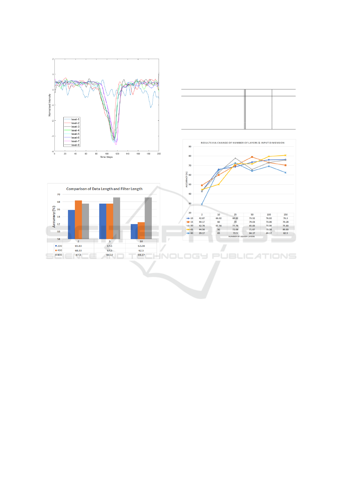
Figure 5: Examples of the normalised LFA time series data

obtained at eight hs-CRP concentration levels.

Figure 6: Comparison of results based on different data

length and ﬁlter window length.

4.4 Dependence with Input Dimension

It was found from the initial testing that the perfor-

mance can be affected by different settings for the

dimension of the mini strips and the number of hid-

den layers. Therefore, we evaluated the performance

by changing these parameters. The dimension of the

mini strip were set as 10, 15, 30, 45 and 90. The

number of input sequences for the LSTM network is

dependent on the dimension of the strip. For exam-

ple, when we treat the mini strip with a dimension 45

as one sequence, then each LFA strip image can be

considered to have 10 sequences. Therefore the total

data for training set is 10 (sequences) × 8 (classes) ×

27 (images) = 2160 and the data size for testing is 10

× 8 × 3 = 240. The number of data samples used for

training and testing under different input arrangement

are given in Table 1. To reduce training time, a data

length of 200 and ﬁlter length of 5 were used. The

performances based on alternative settings are shown

in Figure 7, from which it can be seen that the best

performance is achieved when the input dimension is

45 and number of hidden layers is 150.

Table 1: Data size based on different input dimension.

(Dimension, Sequences) Training Testing

(10, 45) 9720 1080

(15, 30) 6480 720

(30, 15) 3240 360

(45, 10) 2160 240

(90, 5) 1080 120

Figure 7: Comparison of results based on different input

dimension and number of hidden layers.

4.5 Results for Classiﬁcation

The performance of the LSTM for classiﬁcation was

compared to six classiﬁers including SVM, K Near-

est Neighbours (KNN), Linear Discriminant Analysis

(LDA), Decision Tree (DT), Naive Bayes (NB) and

Ensemble. The evaluation was based on different ar-

rangements for input dimensions as shown in Table

1. For fair comparison the same data (partition) was

used to test all algorithms. For LSTM, the data length

was 200 and ﬁlter length was 5. The number of hid-

den layers was selected based on the best performance

from the results in Section 4.4. Since the focus of this

study was to investigate the proposed method based

on LSTM, the default settings in MATLAB were used

for other classiﬁers, such as for Ensemble, the adap-

tive boosting was used for multiclass classiﬁcation.

For KNN the number of neighbours was determined

based on testing the number of neighbours in a range

of 2-8 and the one that gave the best performance was

selected.

The comparison of performance for classiﬁcation

based on different input dimension and number of

Detection and Categorisation of Multilevel High-sensitivity Cardiovascular Biomarkers from Lateral Flow Immunoassay Images via

Recurrent Neural Networks

181

sequences are promising as seen from the Table 2,

which shows that the LSTM outperforms the other

methods in all cases. An example confusion matrix

based on the LSTM (dimension 45, sequence 10) is

given in Figure 8. An example of the Receiver Oper-

ating Characteristic (ROC) curve based on the perfor-

mance from all algorithms is given in Figure 9, which

shows that the LSTM performs better than other clas-

siﬁcation algorithms. The performances for all meth-

ods can be improved, such as by ﬁne tuning parame-

ters via cross validation, or including a third indepen-

dent dataset to chose the optimal number of neigh-

bours in KNN, which will be considered in the next

stage of this work.

Table 2: Comparison of Performance for Classiﬁcation.

Accuracy (%)

Classiﬁers (10,45) (15,30) (30,15) (45,10) (90,5)

SVM 49.35 38.61 58.61 43.33 44.17

KNN 53.43 42.36 49.17 37.92 39.17

LDA 52.50 39.31 53.33 39.58 49.17

DT 54.07 47.92 50.28 45.00 43.33

NB 66.20 58.33 62.60 60.42 57.50

Ensemble 56.30 55.83 65.83 55.42 54.17

LSTM 76.30 73.30 73.33 78.75 76.67

5 DISCUSSION

Over the last decade, many biosensors have been de-

veloped to detect and quantify cardiac biomarkers

in medical diagnostics, in which the signals can be

electrochemical, optical, mass change (piezoelectric /

acoustic wave) or magnetic in nature (Qureshi et al.,

2012). Some of there techniques are relatively de-

manding in terms of sample preparation, costs, analy-

sis times, and skill levels. In contrast, immunoassays

are effective alternatives for rapid screening of sam-

ples, such as the enzyme-linked immunosorbent as-

say (ELISA) and LFA. Main advantages of ELISA are

the possibility to analyse multiple samples simultane-

ously, sensitivity and the relative simplicity. However,

ELISA testing is more time consuming than LFA due

to the operations like repeated incubation, washing

steps and enzyme reaction for ﬁnal signal generation

(Fojt

ıkov

a et al., 2018). The outcomes from this study

are promising which show the improvement of detec-

tion of low concentration biomarkers by LFA using

proposed LSTM networks. For the future work, a

cross-validation can be considered in training to ﬁnd

the optimum parameters for the networks. Techniques

based on the time series analysis or image processing

can be explored for feature extraction before apply-

ing the network, which will potentially improve the

performance.

Figure 8: Confusion matrix for classiﬁcation of eight hs-

CRP concentration levels using LSTM.

Figure 9: Comparison of ROC curve for classiﬁcation.

6 CONCLUSIONS

In this study, a novel method for detection of multi-

level high-sensitivity CRP biomarkers via LFA testing

using LSTM recurrent neural networks is presented.

The proposed methods were evaluated using eight hs-

CRP levels below 5mg/L which is the CRP range for

early risk assessment of CVD. The LFA strip images

were collected from a designed CMOS reader system

under controlled lighting. Each row of an LFA image

is considered as a time series which can be fed to an

LSTM model for classiﬁcation. The dependence be-

tween data length, ﬁlter window length, input dimen-

sion and hidden layers were investigated. The results

show that the proposed LSTM approach achieves bet-

ter performance than other popular machine learning

algorithms although the performance can be further

improved in future work. The preliminary outcomes

BIOIMAGING 2020 - 7th International Conference on Bioimaging

182

are encouraging and suggest the potential of apply-

ing the proposed method for early risk assessment for

CVD.

ACKNOWLEDGEMENTS

This research is carried out under the project of East-

ern Corridor Medical Engineering Centre (ECME)

and funded by the European Unions INTERREG VA

Programme, managed by the Special EU Programmes

Body (SEUPB).

REFERENCES

Carrio, A., Sampedro, C., Sanchez-Lopez, J., Pimienta,

M., and Campoy, P. (2015). Automated low-cost

smartphone-based lateral ﬂow saliva test reader for

drugs-of-abuse detection. Sensors, 15(11):29569–

29593.

Cheung, S. F., Cheng, S. K., and Kamei, D. T. (2015). based

systems for point-of-care biosensing. Journal of lab-

oratory automation, 20(4):316–333.

Choi, J. R., Hu, J., Feng, S., Abas, W. A. B. W.,

Pingguan-Murphy, B., and Xu, F. (2016). Sen-

sitive biomolecule detection in lateral ﬂow assay

with a portable temperature–humidity control device.

Biosensors and Bioelectronics, 79:98–107.

Eltzov, E., Guttel, S., Low Yuen Kei, A., Sinawang, P. D.,

Ionescu, R. E., and Marks, R. S. (2015). Lateral ﬂow

immunoassays–from paper strip to smartphone tech-

nology. Electroanalysis, 27(9):2116–2130.

Fern

andez, S., Graves, A., and Schmidhuber, J. (2007). An

application of recurrent neural networks to discrim-

inative keyword spotting. In International Confer-

ence on Artiﬁcial Neural Networks, pages 220–229.

Springer.

Fojt

ıkov

a, L.,

Sul

akov

a, A., Bla

zkov

a, M., Holubov

a, B.,

Kucha

r, M., Mik

atkov

a, P., Lap

ık, O., and Fukal, L.

(2018). Lateral ﬂow immunoassay and enzyme linked

immunosorbent assay as effective immunomethods

for the detection of synthetic cannabinoid jwh-200

based on the newly synthesized hapten. Toxicology

reports, 5:65–75.

Hochreiter, S. and Schmidhuber, J. (1997). Long short-term

memory. Neural computation, 9(8):1735–1780.

Hu, J., Wang, L., Li, F., Han, Y. L., Lin, M., Lu, T. J., and

Xu, F. (2013). Oligonucleotide-linked gold nanoparti-

cle aggregates for enhanced sensitivity in lateral ﬂow

assays. Lab on a Chip, 13(22):4352–4357.

Hu, J., Wang, S., Wang, L., Li, F., Pingguan-Murphy, B.,

Lu, T. J., and Xu, F. (2014). Advances in paper-based

point-of-care diagnostics. Biosensors and Bioelec-

tronics, 54:585–597.

Jozefowicz, R., Vinyals, O., Schuster, M., Shazeer, N., and

Wu, Y. (2016). Exploring the limits of language mod-

eling. arXiv preprint arXiv:1602.02410.

Mak, W. C., Beni, V., and Turner, A. P. (2016). Lateral-ﬂow

technology: From visual to instrumental. TrAC Trends

in Analytical Chemistry, 79:297–305.

Moghadam, B. Y., Connelly, K. T., and Posner, J. D. (2015).

Two orders of magnitude improvement in detection

limit of lateral ﬂow assays using isotachophoresis. An-

alytical chemistry, 87(2):1009–1017.

Picon, A., Irusta, U.,

Alvarez-Gila, A., Aramendi, E.,

Alonso-Atienza, F., Figuera, C., Ayala, U., Garrote,

E., Wik, L., Kramer-Johansen, J., et al. (2019). Mixed

convolutional and long short-term memory network

for the detection of lethal ventricular arrhythmia. PloS

one, 14(5):e0216756.

Quesada-Gonz

alez, D. and Merkoc¸i, A. (2017). Mobile

phone-based biosensing: An emerging ”diagnostic

and communication” technology. Biosensors and Bio-

electronics, 92:549–562.

Qureshi, A., Gurbuz, Y., and Niazi, J. H. (2012). Biosensors

for cardiac biomarkers detection: A review. Sensors

and Actuators B: Chemical, 171:62–76.

Ridker, P. M. (2003). Clinical application of c-reactive pro-

tein for cardiovascular disease detection and preven-

tion. Circulation, 107(3):363–369.

Ridker, P. M., Hennekens, C. H., Buring, J. E., and Rifai,

N. (2000). C-reactive protein and other markers of

inﬂammation in the prediction of cardiovascular dis-

ease in women. New England Journal of Medicine,

342(12):836–843.

Rivas, L., Medina-S

anchez, M., de la Escosura-Mu

niz, A.,

and Merkoc¸i, A. (2014). Improving sensitivity of gold

nanoparticle-based lateral ﬂow assays by using wax-

printed pillars as delay barriers of microﬂuidics. Lab

on a Chip, 14(22):4406–4414.

Torres, J. L. and Ridker, P. M. (2003). High sensitivity c-

reactive protein in clinical practice. American Heart

Hospital Journal, 1(3):207–211.

Xiong, Z., Nash, M. P., Cheng, E., Fedorov, V. V., Stiles,

M. K., and Zhao, J. (2018). Ecg signal classiﬁcation

for the detection of cardiac arrhythmias using a convo-

lutional recurrent neural network. Physiological mea-

surement, 39(9):094006.

Zeng, N., Wang, Z., Zhang, H., Liu, W., and Alsaadi, F. E.

(2016). Deep belief networks for quantitative analysis

of a gold immunochromatographic strip. Cognitive

Computation, 8(4):684–692.

Detection and Categorisation of Multilevel High-sensitivity Cardiovascular Biomarkers from Lateral Flow Immunoassay Images via

Recurrent Neural Networks

183