A Multi-purpose RGB-D Dataset for Understanding Everyday Objects
Shuichi Akizuki and Manabu Hashimoto
Department of Engineering, Chukyo University, Nagoya, Aichi, Japan
Keywords:
Dataset Generation, Semantic Segmentation, Affordance, 6DoF Pose Estimation.
Abstract:
This paper introduces our ongoing work which is a project of establishing a novel dataset for the benchmarking
of multiple robot vision tasks that aims to handle everyday objects. Our dataset is composed of 3D models,
RGB-D input scenes and multi-type annotations. The 3D models are full-3D scan data of 100 everyday
objects. Input scenes are over 54k RGB-D images that capture the table-top environment, including randomly
placed everyday objects. Our dataset also provides four types of annotation: bounding boxes, affordance
labels, object class labels, and 6 degrees of freedom (6DoF) poses. These are labeled for all objects in an
image. These annotations are easily assigned to images via an original 6DoF annotation tool that has a simple
graphical interface. We also report benchmarking results for modern object recognition algorithms.
1 INTRODUCTION
Achieving human-like tool use using robotic arms is
one of the important goals for intelligent robotics.
Object detection, segmentation and 6 degrees of free-
dom (6DoF) pose estimation are an effective way to
reach this goal. Recent state-of-the-arts deep-learning
techniques have been enabled robot arms to accu-
rately recognize and grasp target objects. For exam-
ple, Single shot multibox detector (SSD) (Liu et al.,
2016) can detect multiple objects in real time from
RGB images. Dex-Net 4.0 (Mahler et al., 2019) can
detect the suitable grasping regions for picking up
randomly stacked objects with a reliability greater
than 95%.
However, these methods are not enough for
human-like tool use. They dont understand the ap-
propriate regions that carry out the specific tasks for
tool use. In the case of the object detection, a robot
can understand the position of a mug as a bounding
box, but it cannot provide information about the re-
gion that could contain liquid.
Understanding the affordance (the functionality of
a parts shape) is also an effective way to achieve
human-like tool use (Do et al., 2018). In the case
of a hammer, the grip part can be used to grasp and
the head part can be used to pound another object.
These parts are used to apply the tasks of grasping and
pounding. Affordance estimation is generally treated
as the semantic segmentation. However, preparing the
training data needs a large amount of time and labor.
In order to solve this problem, we propose a low-
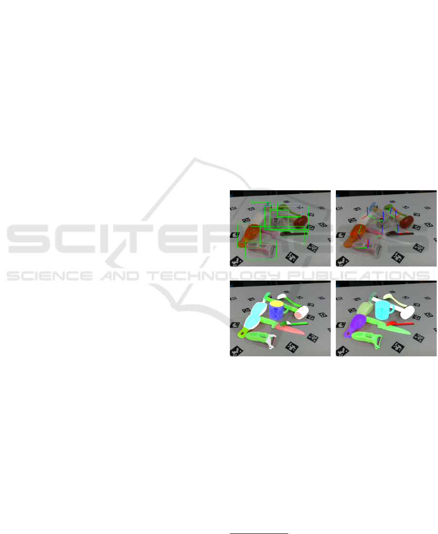
(a) Bounding box (b) 6DoF pose
(c) Affordance label (d) Object class label
Figure 1: Multiple annotations provided by proposed
dataset.
cost annotation procedure for multiple tasks includ-
ing affordance segmentation. And we have devel-
oped a novel dataset by using the proposed method.
The proposed method enables the annotation of four
kinds of information: bounding boxes, 6DoF poses
for each object, pixel-wise object class labels, and the
affordance label shown in figure 2. To the best of
our knowledge, our dataset is the largest that can be
evaluated for multiple tasks including affordance seg-
mentation. The dataset can be downloaded from our
website
1
. In this paper, we report the benchmark-
1
http://isl.sist.chukyo-u.ac.jp/archives/nedopro/
470
Akizuki, S. and Hashimoto, M.
A Multi-purpose RGB-D Dataset for Understanding Everyday Objects.
DOI: 10.5220/0009142504700475
In Proceedings of the 15th International Joint Conference on Computer Vision, Imaging and Computer Graphics Theory and Applications (VISIGRAPP 2020) - Volume 5: VISAPP, pages
470-475
ISBN: 978-989-758-402-2; ISSN: 2184-4321
Copyright
c
2022 by SCITEPRESS – Science and Technology Publications, Lda. All rights reserved

Figure 2: Kitchen and DIY tools.
ing results for object detection and segmentation us-
ing modern deep-learning architectures.
Table 1 summarizes the contents of RGB-D
datasets that can be used for evaluating multiple tasks.
RGB-D Part Affordance Dataset(Myers et al., 2015),
IIT-AFF(Do et al., 2018) and NEDO-v1(Akizuki and
Hashimoto, 2019) are the datasets for the affordance
estimation of tools. They provide pixel-wise affor-
dance labels in each image. IIT-AFF also provides
the bounding box of each tool, and NEDO-v1 pro-
vides accurate 3D models of the tools. However,
these datasets do not have annotations about the 6DoF
poses and the object class labels of each image. There
are many datasets that provide the 6DoF poses of each
object. The LINEMOD dataset(Hinterstoisser et al.,
2012), and the T-LESS dataset(Hoda
ˇ
n et al., 2017)
are famous datasets used for this purpose, but they
dont have affordance information. There is no dataset
that has annotations of multiple tasks, including affor-
dance estimation.
2 PROPOSED DATASET
Our dataset is composed of 3D models of each tool,
input scenes, and annotations.
2.1 Contents
3D Models: Our dataset provides 100 full 3D ob-
ject models which captured actual objects. Table 2
shows the target objects. 10 kinds of kitchen and DIY
tools with 100 instances (see Figure 2) were precisely
modeled using a 3D scanner. The Solutionix C500 3D
scanner from Medit Inc. was used for modeling, and
mesh data comprises of roughly 500,000 vertices for
each object.
Input Scene: Input scenes are the 54,867 RGB-D
images of table-top situations which contain between
5 and 9 (average 6.67) target objects. Image resolu-
tion is 640×480. We randomly chosen and put ob-
jects on the table, and about 550 images of them were
captured by an in-hand RGB-D camera. This proce-
dure were repeated 100 times. We used an Intel Re-
alsense SR305 for capturing all images. Of the im-
ages, 43,831 were for training and the rest were for
testing.
Annotations: Our dataset provides four types of
annotation: bounding boxes, affordance labels, ob-
ject class labels, and 6DoF poses. These are labeled
for all objects in the image. Bounding boxes are pro-
vided as rectangles that tightly surround the objects.
Affordance labels are pixel-wise information that rep-
resent functionally of partial region on the object sur-
face. Table 3 shows the definition of 10 labels (9
classes + background). This definition is same as that
of the paper (Akizuki and Hashimoto, 2019). Object
class labels are pixel-wise information that represent
the object category. Eleven labels (10 classes in Ta-
ble 2 + background) were prepared. A 6DoF pose,
T = [R, t;0, 1], represents the object pose in the input
image. R is a 3 × 3 rotation matrix, and t is a 3 × 1
translation vector. 6DoF pose of all target objects are
provided.
Affordance label 3D model of each target object
are also assigned as color of mesh.
2.2 Statistics
Figure 3 shows the statistics of our dataset. Figure
3(a) shows the number of appearances of each object
class in the scene, which is composed of 100 object
layouts in total. The most frequently appeared object
class, ladle, appeared 93 times, and the least frequent,
hammer, appeared 40 times. The number of frequen-
cies is in proportion to the number of objects for each
class, which is explained in Table 2.
Figure 3(a) and (b) shows the distribution of af-
fordance labels and object class labels. Note that the
label background, which is assigned to other regions
in the image, is ignored in this figure because the fre-
quency is too higher compared to other classes. In
figure 3(b), frequency of the label grasp is relatively
higher than that of others because this label is com-
mon for all objects. The label pound is the least fre-
quent because it is only assigned to the head part of
the hammer. The distribution of the object class label
shown in figure 3(c) represents the area of each ob-
ject class. Therefore, the frequency of large objects
became higher.
A Multi-purpose RGB-D Dataset for Understanding Everyday Objects
471
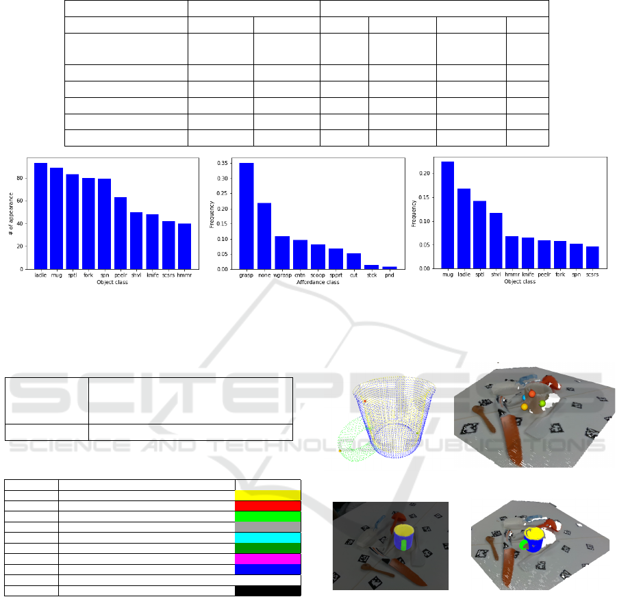
Table 1: List of RGB-D datasets that can be used for evaluating multiple tasks. Due to space limitation, some following
abbreviations are used. (BBox: Bounding box, Aff mask: Affordance mask, Obj mask: Object class mask, Pose: 6DoF pose)
Data Annotation
# images # models BBox Aff mask Obj mask Pose
RGB-D Part
Affordance Dataset
31k – – X – –
IIT-AFF 9k – X X – –
NEDO-v1 10k 72 – X – –
LINEMOD 18k 15 – – – X
T-LESS 49k 30 – – – X
Ours 54k 100 X X X X
(a) Object class wise number of appearances (b) Affordance label distribution (c) Object class label distribution
Figure 3: Dataset statistics. Some class names are abbreviated. (sptl: spatula, spn: spoon, peelr: peeler, shvl: shovel, scsrs:
scissors, hmmr: hammer, wgrasp: wrap-grasp, cntn: contain, spprt: support, stck: stick, pnd: pound.)
Table 2: Object class and the number of 3D models.
Kitchen tool
Fork(11), Knife(6), Ladle(20),
Mug(15), Peeler(9), Spatula(13),
Spoon(12)
DIY tool Hammer(4), Scissors(4), Shovel(6)
Table 3: Affordance labels and corresponding colors.
Affordance Functionality Color
Contain With deep cavities to hold liquid. (255,255,0)
Cut Used for separating another object. (255,0,0)
Grasp Can be enclosed by a hand. (0,255,0)
Pound Used for striking other objects. (160, 160, 160)
Scoop
A curved surface that gathers soft material.
(0, 255, 255)
Stick Sharp parts that can be pushed into something. (0,150,0)
Support Flat parts that can hold loose material. (255,0,255)
Wrap-grasp Can be held with the hand and palm. (0,0,255)
None Other region on objects. (255,255,255)
Background Other region outside of objects. (0,0,0)
3 ANNOTATION PROCEDURE
We used a low-cost annotation procedure (Akizuki
and Hashimoto, 2019) and enhanced it to generate
multi-type annotations for preparing our dataset. This
method allows a semi-automatic process to generate
ground-truth images with pixel-wise annotations for
input images taken from multiple viewpoints. The al-
gorithm consists of three steps, as explained below.
1. 6DoF pose annotation
2. Camera pose estimation using ArUco(Garrido-
Jurado et al., 2014)
(a) Common point picking
(b) Pose refinement by ICP (c) Annotation result
Figure 4: The annotation procedure for 6DoF pose by the
developed software.
3. Ground truth image rendering
In Step 1, the pose of each object in a reference im-
age is manually estimated. We have developed a soft-
ware that enables rapid annotation compared to that
proposed by (Akizuki and Hashimoto, 2019). Fig-
ure 4 shows an interactive annotation procedure using
our software. At first, a user picks more than three
corresponding points from an object model M
i
, i =
{1, ..., n} and a reference image I; these are displayed
on screen by point cloud representation. The picked
VISAPP 2020 - 15th International Conference on Computer Vision Theory and Applications
472

points are shown in 4(a) as colored small spheres.
The software calculates the rigid transformation that
aligns the object model to the input scene by align-
ing the picked points and renders a transformed ob-
ject model on to the input scene as an image repre-
sentation. Users refines the transformation using an
ICP algorithm (Besl and McKay, 1992) by pressing
the key, as shown in 4(b). The final transformation
T
M
i
= [R, t; 0, 1] can be checked via the 3D point cloud
viewer as shown in figure 4(c).
In Step 2, relative camera poses T
C
j
between
the reference image I and the rest of the frames
I
j
, j = {1, ..., n} are calculated by using ArUco li-
brary, which can accurately compute the pose of the
Augmented Reality (AR) markers.
Finally, in Step 3, multiple ground-truth annota-
tions (including bounding boxes, 6DoF poses, affor-
dance labels, and object class labels) are generated
based on the pose data computed in Steps 1 and 2. Ac-
cording to the results of Steps 1 and 2, the pose of the
object M
i
in I
n
can be denoted by T
C
j
T
M
i
. However,
the two transformations may include slight errors that
should be corrected. The object models appearing in
the scene M
i
are merged into a point cloud after ap-
plying the transformation T
C
j
T
M
i
. A transformation
for correction T
r
that minimizes errors between the
merged point cloud and the scene I
j
is calculated by
an ICP algorithm. Therefore, the final transformation
is denoted by T
r
T
C
j
T
M
i
, and is applied for all object
models M
i
.
Annotations are generated by rendering them to
the images of I
j
. As for the affordance and object
class labels, an assigned label of each point of M
i
is
rendered. Bounding boxes are calculated from the
silhouettes of each model. The 6DoF poses of each
model M
i
in an image I
n
is T
r
T
C
j
T
M
i
.
4 EXPERIMENTS
4.1 Annotation Cost
This section discusses the annotation cost of the
proposed annotation software. One importance dif-
ference from the previous method (Akizuki and
Hashimoto, 2019) is Step 1, the 6DoF annotation
shown in figure 4(a). The previous method incremen-
tally transformed the object model via keyboard and
mouse operation. Our method only needs a few cor-
responding points to be picked from an object model
and input scene. It is confirmed that the annotation
cost of this process improved from 15–20 min to 8
min.
4.2 Object Recognition Task: Setting
We have conducted the benchmarking for our dataset
using modern object recognition algorithms. Three
tasks–affordance segmentation, object class segmen-
tation and object detection–were tested. The dataset
was split into a training set and a testing set. Of the
100 layouts, 80 were used as a training set and 20
were used as a testing set. Each set has 43831 and
11036 images, respectively.
4.3 Task 1: Affordance Segmentation
In this experiment, we employed the following seg-
mentation models for comparison.
1. Fully convolutional networks (FCN-8s) (Long
et al., 2015)
2. SegNet(Badrinarayanan et al., 2017)
3. Full-resolution residual networks (FRRN-A
(Pohlen et al., 2017)
We trained each model for 150k iterations at a batch
size of 1. To evaluate recognition performance, we
used intersection over union (IoU), which is widely
used as an index for segmentation tasks. IoU scores
of each method are shown in Table 4. Figure5 shows
the result of affordance segmentation.
Mean IoU score of FRRN-A achieved a higher
score than that of others. IoU scores of affordance
class that have high frequency in figure 3(b) are rela-
tively higher compared with that of the other class.
This was the common tendency of three network
models.
4.4 Task 2: Object Class Segmentation
In this experiment, we used the same algorithms that
were used for Task 1. IoU scores of each method
are shown in Table 5. The classes mug and shovel
were composed of the affordances contain, grasp, and
wrap-grasp, and the IoU scores of these affordance la-
bels were relatively higher in the Task 1 experiment.
Therefore, it seems that the recognition performance
of two kinds of label have a correlation.
4.5 Task 3: Object Detection
In this experiment, we evaluated the performance of
object-detection tasks by comparing mean average
precision (mAP) scores for each object class. We
used SSD (Liu et al., 2016) for this experiment. mAP
scores of each object class are shown in Table 6.
A Multi-purpose RGB-D Dataset for Understanding Everyday Objects
473
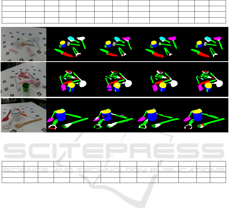
Table 4: IoU score of each affordance segmentation.
Cntain Cut Grasp Pound Scoop Stick Support Wrap-grasp None BG Mean
FCN-8s 0.86 0.47 0.62 0.62 0.55 0.40 0.50 0.77 0.50 0.96 0.63
SegNet 0.62 0.42 0.62 0.33 0.47 0.31 0.00 0.76 0.44 0.96 0.49
FRRN-A 0.88 0.60 0.68 0.67 0.65 0.43 0.54 0.83 0.54 0.96 0.68
(a) Input image (b) Ground truth (c) FCN-8s (d) SegNet (e) FRRN-A
Figure 5: Result of affordance segmentation.
Table 5: IoU scores of object class segmentation.
Fork Knife Ladle Mug Peeler Spatula Spoon Hammer Scissors Shovel BG Mean
FCN-8s 0.49 0.61 0.67 0.87 0.56 0.64 0.65 0.60 0.62 0.77 0.96 0.68
SegNet 0.00 0.58 0.66 0.88 0.00 0.64 0.00 0.00 0.00 0.76 0.93 0.40
FRRN-A 0.41 0.61 0.53 0.90 0.52 0.63 0.50 0.49 0.50 0.77 0.96 0.62
Figure6 shows the result of object class segmen-
tation. It was confirmed that mAP scores of the slen-
der objects (spoon, fork and hammer) were relatively
lower than that of other objects.
5 CONCLUSION
We have proposed a novel dataset for evaluating mul-
tiple robot vision tasks including object detection,
affordance segmentation, object class segmentation,
and 6DoF pose estimation. The dataset contained full
3D scans of 100 object models, 54k RGB-D scenes
and annotation for four kinds of tasks. Our dataset
is the largest that can be evaluated for multiple tasks,
including affordance segmentation, and it is enabled
to train the deep-learning architectures. We have re-
ported the benchmarking results of affordance seg-
mentation, object class segmentation, and object de-
tection. In the near future, we will expand the number
of deep-learning architectures for benchmarking and
will perform the benchmarking of 6DoF pose estima-
tion.
REFERENCES
Akizuki, S. and Hashimoto, M. (2019). Semi-automatic
training data generation for semantic segmentation us-
ing 6dof pose estimation. In International Joint Con-
ference on Computer Vision, Imaging and Computer
Graphics Theory and Applications(VISAPP).
Badrinarayanan, V., Kendall, A., and Cipolla, R. (2017).
Segnet: A deep convolutional encoder-decoder archi-
tecture for image segmentation. IEEE Transactions on
Pattern Analysis and Machine Intelligence.
Besl, P. and McKay, N. (1992). A Method for Registration
of 3-D Shapes. IEEE Transactions on Pattern Analysis
and Machine Intelligence (PAMI), 14(2):239–256.
Do, T.-T., Nguyen, A., and Reid, I. (2018). Affordancenet:
An end-to-end deep learning approach for object af-
VISAPP 2020 - 15th International Conference on Computer Vision Theory and Applications
474
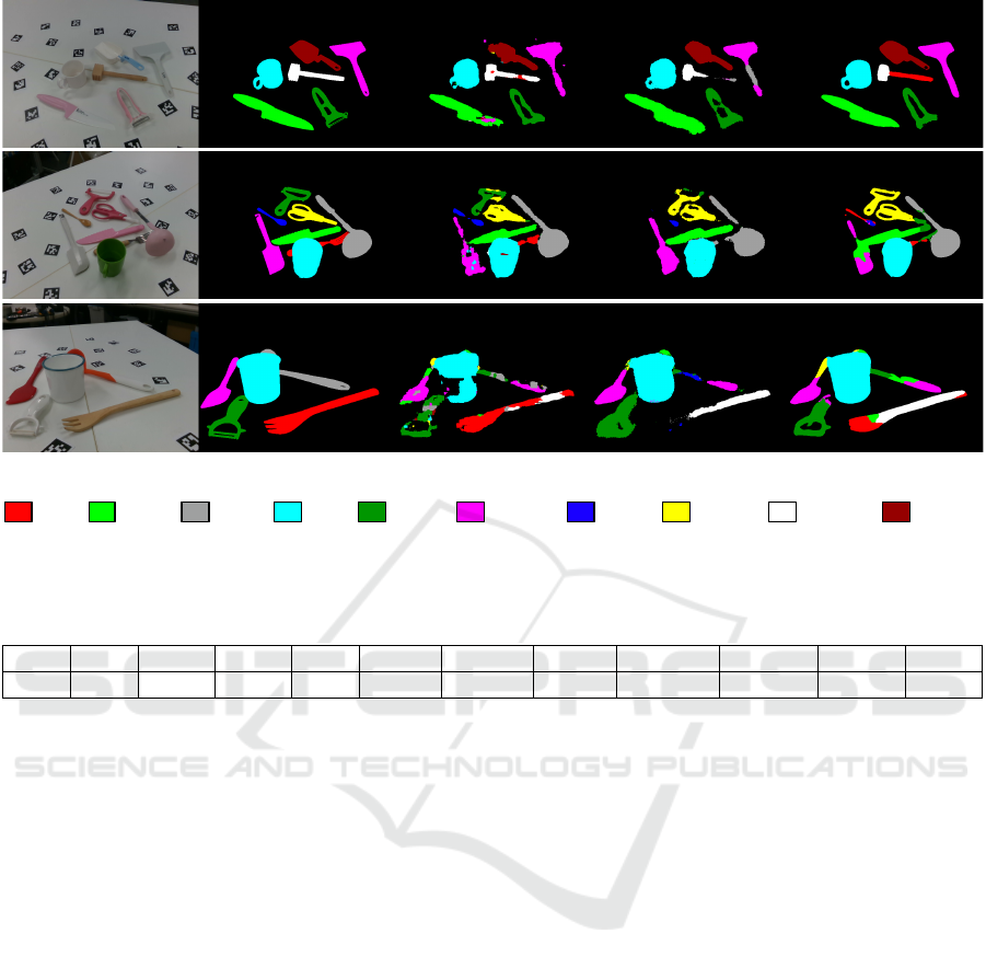
(a) Input image (b) Ground truth (c) FCN-8s (d) SegNet (e) FRRN-A
Fork Knife Ladle Mug Peeler Spatula Spoon Scissors Hammer Shovel
(f) Object class label
Figure 6: Result of object class segmentation.
Table 6: mAP scores of object detection.
Fork Knife Ladle Mug Peeler Spatula Spoon Hammer Scissors Shovel Mean
SSD 0.75 0.84 0.88 0.91 0.88 0.85 0.78 0.79 0.89 0.88 0.84
fordance detection. In International Conference on
Robotics and Automation (ICRA).
Garrido-Jurado, S., Mu
˜
noz Salinas, R., Madrid-Cuevas, F.,
and Mar
´
ın-Jim
´
enez, M. (2014). Automatic generation
and detection of highly reliable fiducial markers under
occlusion. Pattern Recognition, 47(6):2280–2292.
Hinterstoisser, S., Cagniart, C., Ilic, S., Sturm, P., Navab,
N., Fua, P., and Lepetit, V. (2012). Gradient response
maps for real-time detection of texture-less objects.
IEEE Transactions on Pattern Analysis and Machine
Intelligence.
Hoda
ˇ
n, T., Haluza, P., Obdr
ˇ
z
´
alek,
ˇ
S., Matas, J., Lourakis,
M., and Zabulis, X. (2017). T-LESS: An RGB-D
dataset for 6D pose estimation of texture-less objects.
IEEE Winter Conference on Applications of Computer
Vision (WACV).
Liu, W., Anguelov, D., Erhan, D., Szegedy, C., Reed, S.,
Fu, C.-Y., and Berg, A. C. (2016). Ssd: Single shot
multibox detector. In European conference on com-
puter vision (ECCV), pages 21–37. Springer.
Long, J., Shelhamer, E., and Darrell, T. (2015). Fully con-
volutional networks for semantic segmentation. In
Proceedings of the IEEE conference on computer vi-
sion and pattern recognition, pages 3431–3440.
Mahler, J., Matl, M., Satish, V., Danielczuk, M., DeRose,
B., McKinley, S., and Goldberg, K. (2019). Learn-
ing ambidextrous robot grasping policies. Science
Robotics, 4(26):eaau4984.
Myers, A., Teo, C. L., Ferm
¨
uller, C., and Aloimonos,
Y. (2015). Affordance detection of tool parts from
geometric features. In International Conference on
Robotics and Automation (ICRA), pages 1374–1381.
Pohlen, T., Hermans, A., Mathias, M., and Leibe, B. (2017).
Full-resolution residual networks for semantic seg-
mentation in street scenes. In IEEE Conference on
Computer Vision and Pattern Recognition (CVPR).
A Multi-purpose RGB-D Dataset for Understanding Everyday Objects
475
