Learning Efﬁcient Coordination Strategy for Multi-step Tasks in

Multi-agent Systems using Deep Reinforcement Learning

Zean Zhu

, Elhadji Amadou Oury Diallo

and Toshiharu Sugawara

Department of Computer Science and Communication Engineering,

Waseda University, 3-4-1 Okubo, Shinjuku-ku, Tokyo 169-8555, Japan

Keywords:

Multi-agent System, Deep Reinforcement Learning, Coordination, Cooperation.

Abstract:

We investigated whether a group of agents could learn the strategic policy with different sizes of input by

deep Q-learning in a simulated takeout platform environment. Agents are often required to cooperate and/or

coordinate with each other to achieve their goals, but making appropriate sequential decisions for coordinated

behaviors based on dynamic and complex states is one of the challenging issues for the study of multi-agent

systems. Although it is already investigated that intelligent agents could learn the coordinated strategies using

deep Q-learning to efﬁciently execute simple one-step tasks, they are also expected to generate a certain co-

ordination regime for more complex tasks, such as multi-step coordinated ones, in dynamic environments. To

solve this problem, we introduced the deep reinforcement learning framework with two kinds of distributions

of the neural networks, centralized and decentralized deep Q-networks (DQNs). We examined and compared

the performances using these two DQN network distributions with various sizes of the agents’ views. The

experimental results showed that these networks could learn coordinated policies to manage agents by using

local view inputs, and thus, could improve their entire performance. However, we also showed that their

behaviors of multiple agents seemed quite different depending on the network distributions.

1 INTRODUCTION

Learning efﬁcient coordination and cooperation strat-

egy in solving the problems in a complex environment

is a central issue in a multi-agent system. To achieve

this sort of learning, agents are expected to observe

the surrounding environment combined with their in-

ternal states to make appropriate decisions. Although

a number of studies such as (Miyashita and Sugawara,

2019) showed that agents could learn coordinated pol-

icy well for the execution of a simple one-step task

in the environment using the deep Q-learning, intelli-

gent agents need to learn to execute tasks consisting

of a few steps in a cooperative manner. For example,

in a takeout platform environment, such as Uber Eats

and Talabat, delivery agents have to locate restaurants

to pick up ordered dishes ﬁrstly and then deliver them

to the destinations where customers wait. Besides,

being aware of their current state is very important

because they will be unable to take any other future

order for a while if they get a contract of the current

https://orcid.org/0000-0001-9541-4270

https://orcid.org/0000-0001-6441-7719

https://orcid.org/0000-0002-9271-4507

order. To achieve desirable cooperative behavior, all

agents should know what they need to do in the cur-

rent situation; otherwise, agents might be affected by

other agents that have inappropriate behaviors.

The deep reinforcement learning (DRL) has been

proved working in many ﬁelds such as video games

(Mnih et al., 2013) and trafﬁc control (Li et al.,

2016). Because it is impractical to learn appropri-

ate actions in the environment in which a vast num-

ber of observable states exist with traditional algo-

rithms like Q-learning, we also attempt to apply the

DRL to the multi-agent system in our experiments

to solve the coordination/cooperation problems in the

dynamic environment. In addition, Markov game

model (Littman, 1994) has been widely used as a uni-

versal model in the multi-agent deep reinforcement

learning (MADRL) (Egorov, 2016). Training a model

for the multi-agent system is still challenging because

the states of agents and their appropriate actions are

mutually and dynamically affected with each other.

Therefore, we examine whether the DRL can gen-

erate a coordination regime for multi-step tasks, like

takeout problems, without conﬂicting their behaviors.

The function of MADRL used to tackle these prob-

Zhu, Z., Diallo, E. and Sugawara, T.

Learning Efﬁcient Coordination Strategy for Multi-step Tasks in Multi-agent Systems using Deep Reinforcement Learning.

DOI: 10.5220/0009160102870294

In Proceedings of the 12th International Conference on Agents and Artiﬁcial Intelligence (ICAART 2020) - Volume 1, pages 287-294

ISBN: 978-989-758-395-7; ISSN: 2184-433X

287

lems in this paper is to learn to generate appropriate

actions for speciﬁc states to maximize the numerical

rewards for all or individual agents depending on the

deployment of the deep Q-networks (DQNs) for the

DRL. To examine from these perspectives, we intro-

duce two types of training in MADRL; centralized

training, in which a manager has a DQN to be trained

to generate actions for all agents, and decentralized

training, in which individual agents are trained to gen-

erate better actions for themselves. Our contribution

is to examine the performance of these two training

methods and compare the agents’ behavior for multi-

step tasks (i.e., orders) constantly occurring in the en-

vironment.

Furthermore, we also changed the observable

views of each agent for training to see the differences

in the emerging collective behaviors. We developed a

takeout platform simulator in which multi-step tasks

are generated continuously and investigated the effect

of the DQN distribution on the entire performance.

Note that although the size of our simulation environ-

ment is not so large, the number of states for learning

is enormous and the rules in the environment are com-

plex. Nevertheless, our experimental results indicate

that learning by MADRL converged to efﬁcient be-

haviors of multiple agents but their behaviors were

quite different depending on the distribution of the

DQNs.

2 RELATED WORKS

In general, multi-agent reinforcement learning

(MARL) is used so that multiple agents appropriately

cooperate, coordinate or compete with each other

through taking joint actions with the associated

rewards in the given environment. We focus on

the most related and recent work for multi-agent

systems, especially cooperation and coordination,

to accomplish sophisticated coordinated tasks. The

Q-learning algorithm explained in (Watkins and

Dayan, 1992) is the most fundamental method for

MARL problems. (Tan, 1993) showed that the agents

could learn cooperative behaviors independently

with Q-learning in a simulated social environment in

which independent agents did not perform well with

Q-learning in (Matignon et al., 2012). Unfortunately,

traditional learning approaches such as Q-learning

or policy gradient (Silver et al., 2014) result in poor

performance in our study due to the large size of

observable states of our environment.

Meanwhile, (Mnih et al., 2013) indicated that

the online Q-learning method based on deep learn-

ing models could be used to overcome the problems

time t = 0

time t = 2

time t = 10

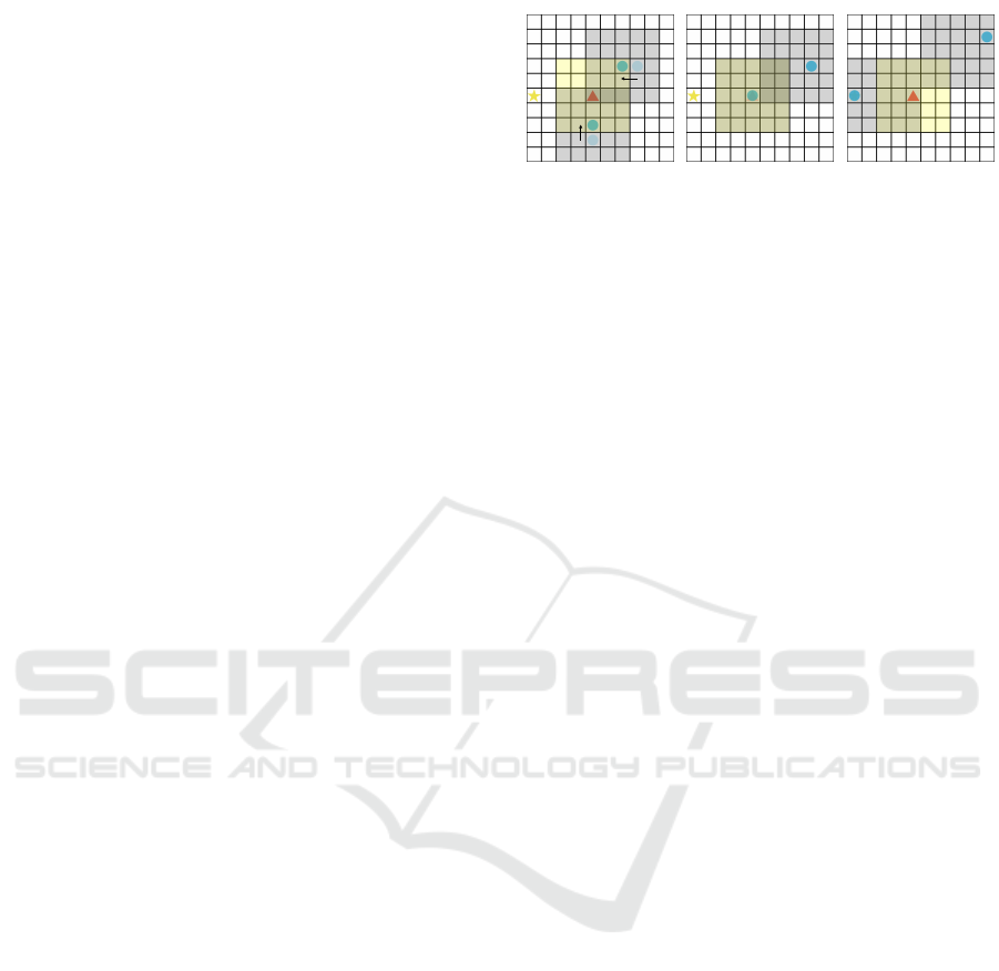
Figure 1: Example Environment with an execution of an

Order.

caused by dynamic environments. Furthermore, sev-

eral ideas have been introduced to make the DQNs

more stable during training procedures. For example,

the experience replay shown in (Mnih et al., 2015)

lets multiple agents remember and reuse experiences

from the past and is the practical method to reduce the

number of transitions required to learn strategies. The

learning algorithms such as DQN and double DQN

(DDQN) (Van Hasselt et al., 2016) architectures are

also used to improve the learning abilities, for exam-

ple, a distributed DDQN framework was applied to

train agents cooperatively move, attack and defend in

various geometric formations (Diallo and Sugawara,

2018).

Moreover, (Lin et al., 2018) used centralized neu-

ral networks to solve the relocation problem in the

large-scale online ride-sharing platform. They pro-

posed a contextual MARL framework in which the

neural network was given additional environment in-

formation when making decisions. However, we have

to mention that the goal of their study was to pre-

dict where agents could take more tasks and agents

would be relocated to destinations instead of explor-

ing destinations by themselves. (Miyashita and Sug-

awara, 2019) compared the coordination regimes as

well as the learning performance with different view

sizes for independent agents. They claim that agents

could learn coordination structures without conﬂicts

with a partial view of the environment, although the

tasks they introduced were the simple one-step tasks,

unlike ours.

3 PROBLEM

We consider a multi-agent problem in which a group

of agents learn the coordinated behavior for delivering

ordered dishes in an online takeout platform. Deliv-

ering tasks are continuously generated by restaurants

according to customers’ requests. When one of the

agents picks up an order from the restaurant and de-

livers the ordered dishes to the customer’s location,

the order is completed. The goal of this problem is to

maximize the order completion rate by agents’ coor-

ICAART 2020 - 12th International Conference on Agents and Artiﬁcial Intelligence

288

dinated behaviors learned with deep neural networks.

Note that a task in our problem consists of two-step

and ordered subtasks; pickup and delivery. An exam-

ple of our problem environment is shown in Fig. 1,

in which the environment is a grid world, red trian-

gles are restaurants, yellow stars are customers, and

blue circles are delivery agents. The possible actions

of agents are one of A = {up, right, down, left}. We

assume that each grid cell has a certain size in which

there can be up to ﬁve agents in it.

When the ordered dishes are almost ready, the

restaurant broadcasts order information to nearby

agents in the broadcast area, which is expressed by

a yellow area in Fig. 1. The restaurant selects and

makes a contract with one of the delivery agents in

this area according to a particular rule, and the se-

lected agent would be guided to this restaurant to

pick up the order. Then, the order will be marked

as the ﬁnished state when the agent arrives at the cus-

tomer’s cell. The agent is expected to learn policy

π that decides where it should wait for future orders

from restaurants, and its actions to deliver the ordered

dishes along with the appropriate path.

We model this problem as a Markov game

N, K, S, A, R

, where N, K, S, A, R are the set of n

agents, the set of restaurants, the set of all local states,

the joint action space, and the reward functions, re-

spectively. The details are given as follows:

• Agent i ∈ N = {1, ..., n}: Agent i is an robot or

delivery person for delivering orders in the take-

out platform.

• Restaurant j ∈ K: Restaurant j will broadcast

orders information to agents in the M × M area

whose center is itself when j has an order to de-

liver. Parameter M is called the broadcast area

size.

• State s

∈ S: Each state is expressed by s

× · · · × s

, where s

is the local state observed

by agent i at time t and contains the information

about the position of itself, the local restaurants

and customers at time t.

• Action a

∈ A: Joint action a

∈ A at time t can be

denoted by the product of all actions a

= (a

··· × a

) ∈ A

× ··· × A

, where A

is the action

space of agent i.

• Reward Function R : R is the function R : S ×

A −→ R, which expresses the reward for joint ac-

tion a

∈ at state s

∈ S

and whose value R(s

, a

)

may be a positive or negative real number.

Fig. 1 shows an example process of delivering an

order. At time t = 0, agent1 (which is denoted by x

this ﬁgure) takes the action to go up and agent2 (x

)

takes action to go left. Then restaurant1 (which is

denoted by r

) broadcasts the request signal about or-

der1 to nearby agents in the yellow area. Both x

and

report their positions to r

. Then, r

selects x

deliver this order because the distance between x

and

is the shortest. From time t = 1 to 2, x

will be nav-

igated by r

to the r

’s cell and given a certain reward

(this reward is +5 in an experiment below) for picking

the order up at t = 2. From time t = 3, x

starts to lo-

cate customer1 (which is denoted by c

in this ﬁgure)

with actions from the deep networks (or random ac-

tions because we will use the ε-greedy learning strat-

egy) until it arrives at c

’s cell. Note that x

cannot

pick up any other order before it completes the cur-

rent order. At time t = 10 in this example, x

reaches

and receives a certain reward (which is +10 in our

experiment below).

4 PROPOSED METHOD

This section describes the methods that were taken in

our experiments to analyze the performance and the

emerging coordinated behaviors by the DQNs. We

applied the centralized DQN and the decentralized

DQNs for learning the agents’ behaviors in a multi-

agent system.

4.1 Decentralized DQNs

The decentralized DQNs mean that agents have their

own deep neural networks whose structures are the

DDQN to generate actions for themselves on the ba-

sis of the local information, in order to achieve their

goals independently. We think that agent i ∈ N will

learn a coordinated strategy through this learning pro-

cess because the appropriate coordination allows it to

maximize its cumulative discounted future reward R

at time t. Note that R

is calculated by

∑

−t

· r

, (1)

where T is the time step at which the simulation envi-

ronment terminates and γ ∈ [0, 1] is the discount factor

that weights the importance of rewards.

Then, the action value of Q for agent i with policy

is deﬁned as

, a

) = E[R

t+1

|s = s

, a = a

], (2)

and the optimal Q

∗

is deﬁned as

∗

, a

) = max

E[R

t+1

|s = s

, a = a

]. (3)

The action-value function for agent i is deﬁned as

∗

, a

) = E[R

t+1

+ γmax

∗

t+1

, a

)|s, a]. (4)

Learning Efﬁcient Coordination Strategy for Multi-step Tasks in Multi-agent Systems using Deep Reinforcement Learning

289

Moreover, the optimal policy of an agent depends not

only on its own states but also on the policies of other

agents. To be more concrete, agents should observe

other agents’ locations and restaurants in their views

to avoid the conﬂicts and redundant activities, such as

gathering in one restaurant, so that they could cooper-

ate to ﬁnish more orders from various restaurants.

At time t, the neural network weight θ

is updated

to minimize the loss function L

(θ

) for agent i, which

is deﬁned as:

(θ

) = E

t+1

)



− Q

, a

;θ

)





, (5)

where y

is the target Q-value of agent i from target

network (Mnih et al., 2015) with parameters θ

i,−

= R

t+1

+ γQ



t+1

, argmax

Q(s

t+1

, a

;θ

i,−

)



(6)

The Q-value for each agent is independent in this

method, and therefore, agents can modify their own

behaviors on the basis of the individual observations.

The state of agent i at time t, s

, is concatenated

with the observations and the distance information.

Note that we use the target Q-network with parame-

ters θ

i,−

updated every P steps to improve the stability

of DQN. P is called the update rate, after this.

4.2 Centralized DQN

The centralized DQN means that there is only one

deep neural network generating actions for all agents

in the environment. In this paper, we consider the case

in which a manager is trained by a neural network

with DDQN structure whose inputs are the collection

(or tensor) of the local states observed by all agents.

Then, the manager attempts to maximize the sum

of the discounted future rewards earned by all agents

at time t, which is deﬁned as

∑

i=1

∑

−t

· r

, (7)

where T and γ are identical to those in Section 4.1.

The action value of Q for all agents with policy π is

calculated by

(s, a) = E[R

t+1

|s = s

, a = a

], (8)

and the optimal Q

∗

for all agents is deﬁned as

∗

(s, a) = max

E[R

t+1

|s = s

, a = a

]. (9)

The action-value function for all agents is deﬁned as

∗

(s, a) = E[R

t+1

+ γmax

∗

t+1

, a)|s, a]. (10)

When optimizing the policy, it should observe the ac-

tions, rewards, and states of all agents. The challenge

Input 1

Input 2

CONV 1 CONV 2 Pooling Flatten FNC 1

FNC 2

Output

(a) Decentralized DQN.

Agent 1

Agent

FCN

FCN 3 FCN 4

Output 1

Output

CONVs

Pooling

Flatten

CONVs

Pooling

Flatten

(b) Centralized DQN.

Figure 2: Neural network architecture.

is to consider and select useful information as input

for training to make all agents work efﬁciently with-

out predeﬁned precise control.

The Q-function is estimated by the network func-

tion approximator with the collection of weights θ of

the network. The network parameters can be updated

by minimizing the loss function L

(θ

) at time t for all

agents:

(θ

) = E

(s,a,r,s

t+1

)



−

∑

i=0

, a

;θ

)





, (11)

where y

is the target Q-value of all agents which is

generated from the target network with parameters

−

= R

t+1

+ γ

∑

i=0



t+1

, argmax

Q(s

t+1

, a

;θ

−

)



(12)

The target network whose parameters θ

−

are up-

dated from the online target network only every P

steps to improve the stability of the output from the

DQN. Two kinds of states, which includes the agent

observations and distance information, are stored to-

gether in the memory pool. In this method, the Q

value is the sum of rewards from all agents to make

sure that all agents can receive appropriate actions

from the manager. When one or a few agents do

not work correctly, the total value of rewards will de-

crease; thus, the deep neural network should be ad-

justed in time.

4.3 Structure of Deep Q Networks

The architecture of the decentralized DQNs used in

our experiments is shown in Fig. 2a. It is composed of

convolution network layers, max-pooling layer, ﬂat-

ten layer, and fully connected network (FCN) layers.

Input1 includes the local view observation by the in-

dividual agents, the order distribution, and the cus-

tomer locations, while Input2 includes the associated

information, such as the distance from the agent to the

customer. The output is four values of actions, i.e., up,

right, down, or left, and the action with the maximum

value is selected (with possibility 1 − ε).

ICAART 2020 - 12th International Conference on Agents and Artiﬁcial Intelligence

290

Fig. 2b shows the centralized DQN architecture

used in our experiments. The convolution layers are

used to maintain spatial relationships between the

states of all agents. The observations from all agents

are collected and processed with the same network

structure shown in Fig. 2a. Then, all of them will be

concatenated into FCN layers (FCNs 3 and 4). Fi-

nally, n outputs which include the values of actions

for all agents, will be generated for the corresponding

agents.

4.4 Reward Structure

We design a reward scheme to encourage agents to be-

have reasonably as well as to accelerate the learning

process. Each time when agents move one step, they

receive a small negative reward −0.01. If they get

stuck in the border of the grid world, which means

they try to get out of the environment, they receive

a negative reward −0.1. When they pick up an or-

der from the restaurant, they receive a positive reward

+5.0. Because it is more difﬁcult for them to deliver

the dishes to the customers’ positions, they will be

given a bigger positive reward +10.0 when they suc-

ceed in arriving in customers’ cells.

4.5 Exploration and Exploitation

Exploration means that agents explore new states by

random actions to improve the policy. On the other

hand, with exploitation, agents select the most opti-

mal action based on past memory. We use ε-greedy

(0 ≤ ε ≤ 1) to make a balance between exploration

and exploitation. At the time t, agents take a random

action with the possibility ε

and take an optimal ac-

tion according to current policy with the possibility

1 − ε

. ε

can be calculated by

= max(ε

init

· φ

, ε

min

where ε

init

is the initial value at time t = 0 and ε

min

the lower bound.

5 EXPERIMENTS

5.1 Experimental Settings

We conducted a number of experiments to compare

the performances of the learned behaviors by us-

ing both the centralized DQN and the decentralized

DQNs with different view sizes of inputs for the neu-

ral networks. The parameters used in our experiments

are listed in Table 1. We set the local view size to

Table 1: Experimental parameters.

Parameter Value

Size of environment 20 × 20

Number of agents (n) 12

Number of restaurants (|K|) 10

Broadcast area size (M) 5

Time steps in one episode 720 time steps

Total number of orders 344 per episode

Initial value of ε (ε

init

) 1.0

Lower bound of ε (ε

min

) 0.1

Decay rate (φ) 0.9999995

Update rate (P) 7200 time steps

Discount factor (γ) 0.95

Figure 3: Training loss value.

(2 × V + 1, 2 ×V + 1) and changed V in the experi-

ments. The takeout simulation environment was ter-

minated when the time step increased to 720, even if

there were remaining orders in the restaurants. The

positions of the agent were scattered in the envi-

ronment randomly at the beginning of each episode

while the positions of restaurants were ﬁxed in all

episodes. Customers whose positions were randomly

determined in the grid world were generated together

with their orders. The positions of customers were

only shown to the agents that have picked up the cor-

responding ordered dishes at the restaurants. Then,

the customers disappeared right after agents arrived

at the customers’ positions. The number of orders in

each episode was 344 because we expect each agent

could complete one order within 25 time steps after

sufﬁcient training. All orders in the experiment had

no time limitation and restaurants would broadcast

orders information when the orders were generated.

All experimental results of the learning methods pre-

sented here are averaged over three runs.

Learning Efﬁcient Coordination Strategy for Multi-step Tasks in Multi-agent Systems using Deep Reinforcement Learning

291

Table 2: Order completion rate in percentage (%) with all

methods for each restaurant.

Centralized DQN Decentralized DQN

V = 6 V = 7 V = 9 V = 6 V = 7 V = 9

Restaurant ID

1 48.16 73.52 86.38 11.81 37.91 54.60

2 98.49 98.12 98.99 75.30 95.48 96.56

3 97.69 97.80 100.00 69.39 98.24 99.26

4 72.83 89.69 97.61 22.78 65.82 76.95

5 98.56 98.62 97.23 78.17 96.70 97.10

6 85.54 95.78 99.38 38.50 86.78 95.63

7 97.89 95.48 97.33 73.14 96.62 98.70

8 93.47 98.48 95.83 78.46 95.90 98.82

9 97.47 95.91 97.27 47.54 88.07 96.01

10 97.76 99.49 98.23 61.30 96.36 97.12

Average 88.79 94.29 96.82 55.64 85.79 91.08

Figure 4: Reward.

5.2 Learning Convergence and Loss

Values

The loss values obtained in our experiments is shown

in Fig. 3. This ﬁgure clearly shows that the learning

process by centralized DQN and decentralized DQNs

with various local view sizes (where V = 6, 7, and 9)

could converge around 2,500 to 4,000 episodes. The

centralized DQN required more time to learn the pol-

icy π probably because the input contains the obser-

vations from all agents, but the loss values of the cen-

tralized DQN became much smaller than those of the

decentralized DQNs. As the value of V increased, the

loss values converged to lower values in both DQNs.

Note that when V = 9, the local view size was 19×19,

which means they could almost see the whole envi-

ronment.

5.3 Rewards

The rewards reﬂecting the results of doing tasks is an

essential factor to investigate the performance of all

Figure 5: Average steps to ﬁnish one order.

agents. Fig. 4 shows the total rewards that all agents

received. As the results of the loss functions in the

previous section, agents with centralized DQN per-

formed better than agents with decentralized DQNs

when V was identical. It is evident that when V = 6,

the performance of agents with decentralized DQNs

was the lowest. Each agent believed that their actions

were appropriate, but the total rewards were lower

than those with the centralized DQN. Besides, they

were more likely to gather in the same area as shown

in Table 2 which is listed the completion rates of order

deliveries requested by restaurants; this is probably

due to the limited observations (V = 6).

When the agents’ view size was large (V = 9), al-

though the learning using the centralized DQN took

longer time to converge, the centralized DQN learned

a better policy π to make most agents cooperate to

achieve more rewards in the environment after 6,000

episodes (Fig. 4). Note that the manager with cen-

tralized DQN could not always learn a good policy

to generate appropriate actions for all agents, while

agents with the decentralized DQNs could always

learn the individual policies, which might not be bet-

ter than those with the centralized DQN, to generate

actions for our problems.

5.4 Behaviors of Agents

Fig. 5 plots the steps to ﬁnish one order during the

training process. At ﬁrst, all of them needed around

650 time steps, which was almost one episode, to ﬁn-

ish an order. Then, most DQNs could generate better

actions to execute orders, resulting in less than 100

time steps per order after around 2000 episodes. Note

that ε ≈ 0.15 around 2000 episodes. As we mentioned

in Section 5.3, agents controlled by the centralized

DQN (V = 9) took more time steps (approximate 5800

episodes) for learning to pick up and deliver ordered

dishes. The agents with centralized DQN required

fewer time steps to complete the orders than those by

ICAART 2020 - 12th International Conference on Agents and Artiﬁcial Intelligence

292

Figure 6: Locations of agents movement from the evaluation experiment.

the decentralized DQNs when their local view sizes

are identical.

After training, we conducted the three experimen-

tal runs using the trained DQNs to observe the emerg-

ing behaviors of all agents. The parameter ε was

set to 0.1 in these experiments. Each experimental

run consisted of ﬁve episodes, and actions taken by

these agents were generated by the resulting neural

networks or the random method. Fig. 6 shows the lo-

cation heat maps of all agents’ movements, meaning

that how many times agents were at each cell. The

color of the cell becomes darker if agents moved to

the cell more times. The red triangles with integers in-

dicate the restaurants with their IDs. We can see that

the right-bottom corner in Fig. 6d, Fig. 6e and Fig. 6f

are much darker than other cells in the environment

when agents used the decentralized DQNs.

We found that a few agents were wandering in this

corner and waiting for requesting signals from two

restaurants nearby. The agents that wait around this

corner for a long time were different in each episode.

This means that all policies learned from the decen-

tralized DQNs could not perform well if agents found

restaurants in the corner. However, this phenomenon

did not appear in the heat maps of the centralized

DQN experiments; agents were trained well and not

suffering from getting stuck in corners. We can also

observe that the agents with both methods learned

strategies to avoid passing through the areas where

there were no restaurants.

The average order completion rate (in percentage)

with all methods for each restaurant are listed in Ta-

ble 2. Because restaurant1 and restaurant4 were lo-

cated near a corner and therefore, it has slightly lower

chances to receive the order from them and the aver-

age length from them to customers were likely to be

longer; thus, their order completion rates were rela-

tively low. On the other hand, other restaurants, such

as restaurants5 and 8, which are located in the cen-

ter of the environment, have higher order completion

rates. The order completion rates always increased if

the local view size V increased in both centralized and

decentralized DQNs.

5.5 Discussion

We can ﬁnd a few interesting phenomena from our

experimental results. First, both the centralized DQN

and decentralized DQNs with partial observations

could be trained well to learn strategies to complete

the established two-step tasks. It is known that the

small size of inputs could accelerate the convergence

speed for DRL but their solution qualities were lower.

When V = 7, the local view size covers around 56% of

the whole environment, the manager with the central-

ized DQN still could learn a good policy π to manage

all agents well.

Second, the quality of learned behaviors by the

centralized DQN was better than that of the decentral-

ized DQNs in terms of total rewards and the resulting

Learning Efﬁcient Coordination Strategy for Multi-step Tasks in Multi-agent Systems using Deep Reinforcement Learning

293

coordinated strategy. One reason is that states of all

agents were observed and aggregated as the inputs to

the central neural network. Thus, it tries to learn the

policy π to help all agents by avoiding to gather in

one place. Agents using the centralized DQN could

cooperate efﬁciently because they could ﬁnd nearby

restaurants and pick up orders immediately after de-

livering orders to customers by helping and receiv-

ing orders from any restaurants. In contrast, although

agents with decentralized DQNs still can learn poli-

cies for executing the tasks, it is hard for them to learn

such coordinated strategy by mutual cooperation, es-

pecially when they only have a small size of obser-

vations. Instead, they focused on a few restaurants to

receive the orders shown and this is the main differ-

ence in their coordinated behaviors by the centralized

and decentralized DQNs.

6 CONCLUSION

We investigated that a certain coordination strategy

could be learned by multi-agent in a dynamic takeout

platform problem. Our experiment results show that

agents with both DQN methods can learn the cooper-

ation strategy efﬁciently, especially for the centralized

DQN method. With the centralized DQN method,

agents controlled by a manager that could get the

states of all agents could have cooperative behaviors

by receiving the orders from any restaurant ﬂexibly.

On the other hand, agents with decentralized DQNs

could also learn strategies for picking up and deliv-

ering orders, but their behaviors were quite different;

they focused on a few speciﬁc restaurants to receive

orders. However, there was an obvious problem that

agents could not learn well with too small observation

area. This is a pivotal issue which we want to focus

on and solve in the future.

We want to extend the size of the simulation envi-

ronment and the number of agents for our future work.

For example, agents are divided into a few teams in a

large environment, and agents are controlled by vari-

ous team leaders. Different teams are expected to be

responsible for an inevitable part of the region with

coordinated strategies.

ACKNOWLEDGEMENTS

This work is partly supported by JSPS KAKENHI,

Grant number 17KT0044.

REFERENCES

Diallo, E. A. O. and Sugawara, T. (2018). Learning strategic

group formation for coordinated behavior in adver-

sarial multi-agent with double dqn. In International

Conference on Principles and Practice of Multi-Agent

Systems, pages 458–466. Springer.

Egorov, M. (2016). Multi-agent deep reinforcement learn-

ing. CS231n: Convolutional Neural Networks for Vi-

sual Recognition.

Li, L., Lv, Y., and Wang, F.-Y. (2016). Trafﬁc signal timing

via deep reinforcement learning. IEEE/CAA Journal

of Automatica Sinica, 3(3):247–254.

Lin, K., Zhao, R., Xu, Z., and Zhou, J. (2018). Efﬁcient

large-scale ﬂeet management via multi-agent deep re-

inforcement learning. In Proceedings of the 24th

ACM SIGKDD International Conference on Knowl-

edge Discovery & Data Mining, pages 1774–1783.

ACM.

Littman, M. L. (1994). Markov games as a framework

for multi-agent reinforcement learning. In Machine

learning proceedings 1994, pages 157–163. Elsevier.

Matignon, L., Laurent, G. J., and Le Fort-Piat, N. (2012).

Independent reinforcement learners in cooperative

markov games: a survey regarding coordination prob-

lems. The Knowledge Engineering Review, 27(1):1–

31.

Miyashita, Y. and Sugawara, T. (2019). Cooperation and co-

ordination regimes by deep q-learning in multi-agent

task executions. In International Conference on Arti-

ﬁcial Neural Networks, pages 541–554. Springer.

Mnih, V., Kavukcuoglu, K., Silver, D., Graves, A.,

Antonoglou, I., Wierstra, D., and Riedmiller, M.

(2013). Playing atari with deep reinforcement learn-

ing. arXiv preprint arXiv:1312.5602.

Mnih, V., Kavukcuoglu, K., Silver, D., Rusu, A. A., Veness,

J., Bellemare, M. G., Graves, A., Riedmiller, M., Fid-

jeland, A. K., Ostrovski, G., et al. (2015). Human-

level control through deep reinforcement learning.

Nature, 518(7540):529.

Silver, D., Lever, G., Heess, N., Degris, T., Wierstra, D., and

Riedmiller, M. (2014). Deterministic policy gradient

algorithms.

Tan, M. (1993). Multi-agent reinforcement learning: Inde-

pendent vs. cooperative agents. In Proceedings of the

tenth international conference on machine learning,

pages 330–337.

Van Hasselt, H., Guez, A., and Silver, D. (2016). Deep re-

inforcement learning with double q-learning. In Thir-

tieth AAAI conference on artiﬁcial intelligence.

Watkins, C. J. C. H. and Dayan, P. (1992). Q-learning. Ma-

chine Learning, 8(3):279–292.

ICAART 2020 - 12th International Conference on Agents and Artiﬁcial Intelligence

294