
Pedestrian Head and Body Pose Estimation with CNN in the Context of
Automated Driving
Michaela Steinhoff
1
and Daniel G¨ohring
2
1
Business Area Intelligent Driving Functions, IAV GmbH, Rockwellstr. 3, 38518 Gifhorn, Germany
2
Institute of Computer Science, Freie Universit¨at Berlin, Arnimallee 7, 14195 Berlin, Germany
Keywords:
Automated Driving, Convolutional Neural Network, Headpose, Pedestrian Intention, Semi-supervision.
Abstract:
The challenge of determining pedestrians head poses in camera images is a topic that has already been re-
searched extensively. With the ever-increasing level of automation in the field of Advanced Driver Assistance
Systems, a robust head orientation detection is becoming more and more important for pedestrian safety. The
fact that this topic is still relevant, however, indicates the complexity of this task. Recently, trained classi-
fiers for discretized head poses have recorded the best results. But large databases, which are essential for
an appropriate training of neural networks meeting the special requirements of automatic driving, can hardly
be found. Therefore, this paper presents a framework with which reference measurements of head and upper
body poses for the generation of training data can be carried out. This data is used to train a convolutional
neural network for classifying head and upper body poses. The result is extended in a semi-supervised manner
which optimizes and generalizes the detector, so that it is applicable to the prediction of pedestrian intention.
1 INTRODUCTION
The research on automated driving is more relevant
than ever. Semi-automated functions such as auto-
matic parking or driving in stop-and-go traffic have
long been available in the form of assistance systems
(parking and traffic jam assistant). Even fully auto-
mated driving is no longer limited to motorway sce-
narios. Many projects, like Stimulate
1
in Berlin, mas-
ter the challenges of urban traffic already completely
autonomous, although limited in speed. This work is
part of a project, which is contributing to the ongoing
development of self-driving cars.
One of the biggest challenges in urban scenarios is
the robust prediction of pedestrians. Simple tracking
and adapted motion models are not sufficient to map
the highly dynamic behaviour of humans. Therefore,
countless research groups try to extract more infor-
mation from the human posture. In addition to a more
precise analysis of the leg positions, many researchers
also focus on the head pose. Kloeden et al. (2014)
have already shown that the head pose is suitable as a
characteristic for predicting the movements of pedes-
trians. They proved that pedestrians show a protec-
tion behaviour particularly before crossing the road,
1
https://www.wir-fahren-zukunft.de
which can be attached to the increased head move-
ment. For many decades, classical machine learning
has been used to extract this orientation of the head. A
common methodology is the quantification of the an-
gular ranges, and thus the declaration of a classifica-
tion problem (Schulz and Stiefelhagen, 2012). In that
work, the authors scan the upper part of a pedestrian
image, assuming the head to be there. Eight classi-
fiers are used to locate the head within this part and
estimate an initial pose. These classifiers are trained
for eight different head pose classes, each with a
range of 45
◦
. For the continuous estimation of poses,
regression is the preferred method. Lee et al. (2015)
and Chen et al. (2016) extract gradient based charac-
teristics like HOG (Histogram of Oriented Gradients)
features and then use a SVR (Support Vector Regres-
sor) to estimate the head pose.
All these methods only consider the yaw angle of
the head. Contrary to this, the approaches of Reh-
der et al. (2014), Chen et al. (2011) and Fanelli et al.
(2011) take additional orientation directions into ac-
count. The latter receives 3D data from a depth cam-
era and uses it to find the position of the tip of the nose
as well as the yaw, pitch and roll angles of the head
using a Random Regression Forest. A disadvantage
of this method is therefore that only a limited area of
the possible head poses, namely the one with a visible
Steinhoff, M. and Göhring, D.
Pedestrian Head and Body Pose Estimation with CNN in the Context of Automated Driving.
DOI: 10.5220/0009410903530360
In Proceedings of the 6th International Conference on Vehicle Technology and Intelligent Transport Systems (VEHITS 2020), pages 353-360
ISBN: 978-989-758-419-0
Copyright
c
2020 by SCITEPRESS – Science and Technology Publications, Lda. All rights reserved
353

nose, can be determined. It is furthermore assumed
that the head was detected in the image in advance.
Conversely, in Reh-der et al. (2014) monocular RGB
images serve as input data, which do not have to be re-
stricted to the head section, but can contain complete
as well as covered pedestrians. The head localiza-
tion is done within the algorithm via HOG/SVM and
a part-based detector proposed by Felzenszwalb et al.
(2010). Proceeding from this, four discrete classes are
defined for the pose estimation, for each of which a
classifier is trained using logistic regression with LBP
(Local Binary Pattern) features. By integrating the
discrete orientation estimates using a HMM (Hidden
Markov Model), they obtain continuous head poses.
This approach is particularly interesting in that the
head poses are plausibilized and impossible poses are
discarded with the help of the upper body pose and
the motion direction. Chen et al. (2011) go one step
further and estimate both the head and body poses in
pedestrian images. Therefore, the orientation of the
body is divided into eight discrete direction classes
and multi-level HOG features are extracted. Further-
more, the yaw angle range of the head is divided into
twelve classes and the pitch angle range of the head
into three classes. After localizing the head, texture
and color features are extracted by another multi-level
HOG descriptor and histogram-based color detector.
A particle filter framework is subsequently used to
estimate the body and head poses. The dependency
between the poses as well as the temporal relation-
ship are taken into account. Another approach also
estimates both the head and body pose (Flohr et al.,
2015). For both poses, eight orientation-specific de-
tectors are trained, whose class centers are shifted by
45
◦
each. To locate the exact body and head position
in the image, they make use of disparity information
obtained from the stereo input data. Based on this, a
DBN (Dynamic Bayesian Network) is used to get the
current orientation states. Thereby the current head
pose depends on the previous head pose and also on
the current body pose.
Recently, (deep) neural networks have become in-
creasingly important and their application also aims
for an improvement of the head pose detection. Lat-
est nets as presented in (Patacchiola and Cangelosi,
2017) or (Ruiz et al., 2017) predict yaw, pitch and roll
angles in a continuously manner and achieve great ac-
curacy. The input, however, is also here only the head
section, which must be available in relatively high res-
olution. If these approaches are to be used in the con-
text of automatic driving, pedestrians and their head
positions must be recognized early, i.e., from a great
distance, so that the poor quality of the input data does
not fulfill the requirements of the mentioned meth-
ods. The present work, therefore, presents a neural
network that recognizes head poses from images with
the quality of cameras commonly used in vehicles.
Not only the head but the entire pedestrian’s image
section serves as input, since the head pose in rela-
tion to the upper body provides further important in-
formation. From this it can be deduced, for exam-
ple, whether a pedestrian shows a safety behaviour,
which is a clear indication of the intention to cross
the road. For the training of this head and upper body
pose detector, commonly available data sets for head
poses and pedestrians in general like Human3.6m
2
,
PETA
3
or INRIA
4
cannot be used, because the ref-
erence to the upper body alignment is missing. In
addition, most researchers only consider yaw angles
in the range of −90
◦
to 90
◦
, i.e., the frontal view of
the pedestrian heads. In the present project, however,
it is just as important whether a passer-by perceives
oncoming traffic or the automated driving vehicle.
Therefore, a framework for the generation of a ”full-
range” data set will be briefly presented here. Using
a semi-supervised approach, a trained convolutional
neural network (CNN) is extended so that the com-
paratively small amount of self-generated annotated
data is enriched by many unlabeled data from real
test drives within the project and the detector achieves
more accurate results.
The contributions of this work can be summarized in
the following key points:
• a framework for generating a data set with head
and upper body poses,
• training and evaluation of a network (CNN) using
the data set,
• enhancement of training data with real driving
data,
• evaluation of an approach to semi-supervised
learning and improvement of the network.
The paper is structured as follows:
After the second chapter presented the framework
for data set generation, Chapter 3 gives a detailed de-
scription of our detector design. The obtained results
are illustrated in the following chapter. Chapter 5
draws a conclusion and presents an outlook for future
work.
2
http://vision.imar.ro/human3.6m/description.php
3
http://mmlab.ie.cuhk.edu.hk/projects/PETA.html
4
http://pascal.inrialpes.fr/data/human
VEHITS 2020 - 6th International Conference on Vehicle Technology and Intelligent Transport Systems
354

Logging of time,
camera images,
3D object position,
head/body pose
head and body
orientation
time sync., calibration
measurement control
Figure 1: The used framework setup for data set generation.
2 DATA SET GENERATION
As already mentioned, this work requires data that
is not annotated in the common pedestrian data sets.
The added value lies in the fact that not only the pose
of the head, but also that of the upper body in relation
to the head is considered. In order to annotate such
data automatically, a data generation setup and soft-
ware framework was developed which can be applied
to capture images of pedestrians together with the cor-
responding head and upper body poses. Therefore
this section first explains the experimental setup and
the processing infrastructure after that. An overview
of the framework setup is given in Figure 1.
2.1 Experimental Environment
The images were taken by a camera installed in a test
vehicle alongside other sensors such as Lidar. The ve-
hicle was also equipped with an object tracking mo-
dule, which outputs 3D positions of the pedestrians in
vehicle coordinates. Two inertial sensors (MPU6050)
with 6 degrees of freedom each were used to mea-
sure the exact head and upper body orientations. To-
gether with one microcontroller with integrated WiFi
module (ESP8266− 12F) each, these were placed on
the head and upper body of the test persons. Since the
position and orientation of the MPU6050s on the head
and body depend a lot on the probands and the up-
coming measurement, an online calibration was per-
formed at the beginning of each exposure and the sen-
sor values were transformed into quaternions relative
to the corresponding initial pose. In addition, IMU
(inertial measurement unit) drift compensation was
carried out beforehand and the drift behavior was an-
alyzed in the following. With an average duration of
the measurement sequences of 2 minutes, the drift of
0.5
◦
per minute was negligible.
2.2 Processing Infrastructure
The control of the IMU, the online calibration and the
time synchronization via ntp server were realized in
Arduino on the microcontrollers. The measured poses
and the related timestamps were sent via TCP to a log-
ging computer where they were processed and added
to the data set. A single date then consists of the
timestamp with corresponding image, the 3D object
position and yaw, pitch and roll angles of either head
and the upper body. A total of 2500 test and training
data was annotated, including recordings of 20 differ-
ent people at different times of the day and year.
3 HEAD AND UPPER BODY POSE
DETECTOR
This section introduces the developed head pose de-
tector. First of all, the definition of the individual
classes is discussed. The training process is divided
into the two parts supervised and its unsupervised ex-
tension, which are explained in the following two sub-
chapters.
3.1 Class Definition
The detector presented in this paper is intended to de-
tect the yaw angles of the head and upper body. Since
we want to address a classification problem, the an-
notated data has to be mapped to classes. Therefore,
the possible head poses in the range [−105
◦
,105
◦
] are
quantized in α
H
= 30
◦
steps, whereby a yaw angle of
0
◦
implies the head pointing directly towards the cam-
era. All following angles are specified in this defini-
tion of coordinate system.
45°
-45°
15°
-15°
75°
-75°
105°
-105°
155°-155°
Figure 2: The head pose range is divided into 10 classes.
Pedestrian Head and Body Pose Estimation with CNN in the Context of Automated Driving
355

The range ]105
◦
,180
◦
] ∪ [−180
◦
,−105
◦
[ (i.e., facing
away from the camera) is divided into three parts ´a
α
H2
= 50
◦
. Accordingly there are n
hc
= 10 head
classes in total (see Figure 2). For anatomical rea-
sons, the deviation of the upper body pose from the
head pose is limited to a range of −90
◦
to +90
◦
. This
area is divided into n
bc
= 3 body classes C
B
depend-
ing on the head pose. The body either points left
(C
B
= 0), right (C
B
= 2) or in the same direction as
the head (C
B
= 1). This results in an overall number
of 30 classes for the detector. The output classC
out
re-
sulting from the head (C
H
) and upper body (C
B
) class
is calculated according to Eq. 1. The head and upper
body class are derived from the respective yaw angles
ψ
H
and ψ
B
.
C
out
= C
B
· n
hc
+C
H
(1)
with
C
H
=
⌊
ψ
H
−
1
2
α
H
α
H
⌉ +
n
hc
2
, if − 105
◦
≤ ψ
H
≤
α
H
2
⌊
ψ
H
−
1
2
α
H
α
H
⌉ +
n
hc
2
+ 1 , if
α
H
2
< ψ
H
≤ 105
◦
⌊
ψ
H
−
1
2
α
H2
α
H2
⌉ +
n
hc
2
− 1 , if ψ
H
< −105
◦
⌊
ψ
H
−
1
2
α
H2
α
H2
⌉ +
n
hc
2
+ 1 , if 105
◦
< ψ
H
≤ 155
◦
0 , otherwise
(2)
and
C
B
= ⌊
δψ
α
B
+
1
2
⌉ + ⌊
n
bc
2
⌉ (3)
where
δψ =
ψ
H
− ψ
B
+ 360
◦
, if ψ
H
− ψ
B
< −180
◦
ψ
H
− ψ
B
− 360
◦
, if ψ
H
− ψ
B
> +180
◦
ψ
H
− ψ
B
, otherwise
(4)
3.2 Semi-supervised Learning with
CNN
In the domain of neural networks, CNN have been es-
tablished to handle classification tasks. Most of the
best-known classification networks are trained in a
supervised manner with a large amount of annotated
data. Since the present use case makes different de-
mands on the annotation, only the few self-generated
data are available in comparison. The idea to train a
reliable classification network from it nevertheless is
based on a semi-supervised approach.
Figure 3: Samples of unlabeled data, the first row shows
unsorted, the second and third row clustered samples.
Supervised Learning
As mentioned above, CNN are very well suited to
solving classification problems and there are many
proven network architectures. Hence, a CNN is also
used here and the layer topology is oriented to these
architectures. Figure 4 shows a schematic representa-
tion of the underlying network structure.
The input data is scaled to a fixed size (128x128)
and converted to grayscale values. They subsequently
pass through three consecutive blocks each with three
convolutional and one maxpooling layer until a fully
connected layer maps them to an embedding vector
with size 64, which is transformed to logit class scores
by a final dense layer. During training, a dropout layer
located between the last two fully-connected layers
was used with a dropout rate of 0.5 in order to gener-
alize the learning result. To find the best hyper param-
eters for the training, a grid search was applied. Ac-
cordingly, the following parameter configuration pro-
vides the best performance and has been used further:
Table 1: Best parameters found by grid search.
batchsize 50
initial learning rate 0.0001
learning rate decay 0.33
decay steps 10000
optimizer Adam
loss function Cross Entropy
The loss function of the supervised part with labels λ
and predicted outputs y is given by
loss
logit
= −
∑
x
λ· log(y+ 1e
−8
). (5)
VEHITS 2020 - 6th International Conference on Vehicle Technology and Intelligent Transport Systems
356

128
3
128
3
3
128
32
128
3
3
3x Conv K:32, F:3
64
64
64
MaxPooling S:2
3x Conv K:64, F:3
256
32
32
3
3
MaxPooling S:2
3x Conv K:128, F:3
MaxPooling S:2
Flattening
FullyConnected size:64
Dropout KP:0.5
128
32
32
MaxPooling S:2
3x Conv K:256, F:3
3
3
3
3
64
1
Figure 4: Schematic representation of the used network architecture.
Semi-supervised Extension
Due to the comparably small variance of the training
data, the network performed well on similar testing
data. With the aim of optimizing and generalizing
the network, it was extended to include unsupervised
learning. In general, as with most semi-supervised
methods, the results of supervised learning are im-
proved by clustering the unlabeled data and then as-
signing them to already trained classes. Inspired by
the concept of Haeusser et al. (2017), the assignment
is not based on the last but the penultimate layer. In
this so-called ”embedding” level, the similarity of all
unlabeled data to the labeled data is determined. An
actual assignment of the unlabeled data only takes
place if it has been attributed to the same class la-
bel twice due to the highest similarity. To find a suit-
able scale for this similarity, different metrics were
tested and compared to each other. The following
two metrics have emerged as the ones with the best-
performing results.
The cosine similarity describes the correspon-
dence of the orientations of two vectors to be com-
pared. For this purpose the cosine of the angle be-
tween them is determined according to Eq. 6.
cos(θ) =
a· b
kakkbk
(6)
The resulting value range for this scale is therefore
limited to [-1, 1], where ’1’ means that the orientation
of both vectors is identical (θ = 0
◦
). ’-1’ however de-
notes an opposite orientation (θ = 180
◦
) and ’0’ signi-
fies the vectors are orthogonal to each other (θ = 90
◦
).
Aside from being independent of the vectors mag-
nitudes, this metric has the advantage that it is very
computation-performant, since only the dot product
has to be calculated. The loss is determined analogue
to Haeusser et al. (2017) by comparing the resulting
association probability with the expected probability
distribution using cross entropy.
The Mahalanobis distance indicates the distance of a
data point to the mean of a point distribution of one
class in multiples of the standard deviation. Thus, in
contrast to the Euclidean distance, the correlation be-
tween the data points is taken into account and the
assignment to individual clusters of data (classes) be-
comes more accurate.
If~x is a data point to be assigned and~µ is the mean
value of the data set of a class with covariance matrix
C, the Mahalanobis distance is given by:
D
M
(~x) =
q
(~x−~µ)
T
C
−1
(~x−~µ) (7)
The result initially expresses the dissimilarity of the
sample to the data set. By scaling to the value range
D
Ms
= [0,1], reverting the range and normalizing the
multiplication of this association probability with its
transposed the following probability distribution is
obtained stating that several unlabeled data points are
associated with the respective classes:
p = ||(p
A
· p
T
A
)||
2
(8)
with
p
A
= 1− D
Ms
(9)
The expected probability distribution p
E
in this case
is equal to the unit matrix with rank n
C
(number of
classes), since a sample is to be assigned uniquely to
one class. For this purpose it must be ensured that
each class is represented with at least one sample per
batch in the set of unlabeled data. This is achieved
by adding one labeled sample for each class to the
batch with unlabeled samples. The total loss is finally
calculated by applying cross entropy on these proba-
bilities and adding the result to the logit loss from the
supervised part (see Eq.5).
loss = −
∑
x
p
E
· log(p
A
+ 1e
−8
) + loss
logit
(10)
Pedestrian Head and Body Pose Estimation with CNN in the Context of Automated Driving
357

Table 2: Train error, test error, average precision (AP), average recall (AR) and test error including ’adjacent classes’ (TE*)
of SUP, COS and MAHA in [%]. The last two columns declare the distribution of train and test samples within the supervised
and the semi-supervised methods.
train err test err AP AR TE* train samples test samples
SUP 0.17 82.19 16.96 18.27 54.86 2000 500
COS 30.59 66.55 32.57 25.17 43.52 12000 500
MAHA 0.41 58.53 32.26 30.21 32.15 12000 500
Figure 5: Precision and recall of the trained networks, the results of the semi-supervised approaches (COS and MAHA)
improve the supervised one (SUP).
4 EXPERIMENTS
For the training of the head pose detector 2500 la-
beled and 10000 unlabeled data were used. It was
performed on a computer with four GTX 2080 Ti
with 12 GB memory each. Because of the high im-
balance of the class distribution in the labeled train-
ing data set, the maximum number of samples used
per class in all three trainings was limited to avoid
overfitting of more frequent classes. This was al-
ready recommended by Weiss and Provost (2001),
who showed that an unequal distribution does not
usually lead to the best performance. In the follow-
ing, the results of the purely supervised trained net-
work (further referred to as SUP) and the two differ-
ent methods for estimating similarity within the semi-
supervised trained network (MAHA for the one using
the mahalanobis distance, COS for the cosine similar-
ity) are compared. Due to the small number of labeled
samples, SUP converged comparatively quickly after
about 500 epochs. With the best parameters found
by the grid search, a training error of 0.17% was
achieved. But the evaluation with test data confirmed
that the network specialized in the training data. The
error rate for the randomly distributed test data was
82.19% at best (see Table 2).
In the approach of association using cosine simi-
larity, it was necessary that each class is represented in
each batch of labeled data so that each unlabeled sam-
ple can be assigned properly as well. Depending on
the number of samples used per class per batch, this
results in very large batch sizes for 30 classes, which
caused memory issues. But with 10 samples per class
per batch a suitable compromise between training ef-
ficiency and executability was found. This of course
led to a declining of the obtained network accuracy,
resulting in a training error of about 30%. Never-
theless, this as well as the second semi-supervised
VEHITS 2020 - 6th International Conference on Vehicle Technology and Intelligent Transport Systems
358
solution MAHA reduces the test error by a relevant
amount, which is also reflected in Figure 5, depict-
ing the precision and recall per class of all three ap-
proaches. Even if individual classes perform worse
for COS and MAHA than for SUP, the average pre-
cision (AP) and recall (AR) noticeably are higher as
can be seen in Table 2. And although MAHA also
required restrictions in parameter selection due to the
limited memory capacity, this approach yielded the
lowest test error of 59.17%. The fact that the semi-
supervised approaches generalize the training result
and thus enhance it is particularly evident when the
confusion matrix is analyzed more closely. Therefore
Figure 6 illustrates the confusion matrix of MAHA.
For comparison, those of SUP and COS can be found
in the appendix. First of all, it is conspicuous that test
samples of other classes are assigned more often to
the columns 10 to 19, which correspond to the classes
with the same alignment of head and upper body. This
is probablydue to the fact that this natural human pose
occurs more frequently in the unlabeled data set and
thus their training was more effective. Furthermore,
the principal diagonal is highlighted in dark blue as
these cells map the amount of true positives. Accord-
ing to the class definition in Section 3, the classes
ending with the same number (e.g. 3, 13 and 23)
represent the same head class. These cells are also
shaded light blue. The remaining cells are marked
darker gray the higher their cell value is. Mainly in
contrast to the confusion matrix of SUP (see Figure
8), whose predictions are highly scattered, an orienta-
tion of the predicted classes to the principal diagonal
as well as partially to the secondary diagonals of the
same head classes can be observed here.
Figure 6: Confusion matrix of MAHA, rows index the pre-
dicted and columns the actual classes.
In addition, cells of adjacent classes, i.e., those which
differ only in the head pose by a maximum of 30
◦
,
were colored green. It becomes plausible that a high
percentage of test samples are associated with these
cells regarding the fact that these small differences are
difficult to detect, as can be seen in Figure 7. Consid-
ering this in the error calculation and including the ad-
jacent classes in the set of correct predictions, results
in the test error listed in Table 2 under TE*, which for
MAHA is only 32.15%.
Figure 7: Prediction example, Left: a sample incorrectly
predicted as class 14, Right: an actual sample of class 14.
5 CONCLUSIONS
In this paper, a head pose detector was presented that
meets the special requirements of automated driving.
Since the relative pose of the upper body was of im-
portance in the project within which the work was de-
veloped, in addition to the pure yaw angle of the head,
a new data set was generated. Conceived for this pur-
pose, a reference data measuring setup with software
framework was used to generate data for training and
evaluating a neural network. Due to the relatively
small amount of data, the performance of this purely
supervised trained classifier was, as expected, poorly.
Therefore, the data set was enriched by the numerous
unlabeled data available from test drives in the project
and an approach of semi-supervised learning was de-
veloped and optimized. The test result was thus im-
provedby almost 25%. Furthermore, it was found that
many of the misclassifications were associated with
the so-called adjacent classes. In the context of auto-
mated driving, one of the strongest motivations for the
detection of head poses is the assessment of whether a
pedestrian has perceived the driving vehicle or not. It
could be demonstrated that the small pose differences
between two adjacent classes are often very difficult
to identify and have little influence on the determina-
tion of whether the vehicle was seen or not. An ad-
justed test error of only about 32% could be reported.
Pedestrian Head and Body Pose Estimation with CNN in the Context of Automated Driving
359

Overall, it was found that the semi-supervised
method used is very well suited to improve the perfor-
mance of the head pose detector despite a small data
set. In the future, further result optimizations can be
achieved by more labeled training data. In addition,
better performance will be obtained by upgrading the
computer’s performance and memory capacity.
REFERENCES
Chen, C., Heili, A., and Odobez, J. (2011). A joint esti-
mation of head and body orientation cues in surveil-
lance video. In 2011 IEEE International Conference
on Computer Vision Workshops (ICCV Workshops),
pages 860–867.
Chen, J., Wu, J., Richter, K., Konrad, J., and Ishwar, P.
(2016). Estimating head pose orientation using ex-
tremely low resolution images. In 2016 IEEE South-
west Symposium on Image Analysis and Interpretation
(SSIAI), number 1, pages 65–68. IEEE.
Fanelli, G., Gall, J., and Van Gool, L. (2011). Real time
head pose estimation with random regression forests.
In Computer Vision and Pattern Recognition (CVPR),
2011 IEEE Conference on, pages 617–624. IEEE.
Felzenszwalb, P. F., Girshick, R. B., McAllester, D., and
Ramanan, D. (2010). Object detection with discrim-
inatively trained part-based models. IEEE Transac-
tions on Pattern Analysis and Machine Intelligence,
32(9):1627–1645.
Flohr, F., Dumitru-Guzu, M., Kooij, J. F. P., and Gavrila,
D. M. (2015). A probabilistic framework for joint
pedestrian head and body orientation estimation.
IEEE Transactions on Intelligent Transportation Sys-
tems, 16(4):1872–1882.
Haeusser, P., Mordvintsev, A., and Cremers, D. (2017).
Learning by association - a versatile semi-supervised
training method for neural networks. In IEEE Con-
ference on Computer Vision and Pattern Recognition
(CVPR).
Kloeden, H., Brouwer, N., Ries, S., and Rasshofer,
R. (2014). Potenzial der Kopfposenerkennung
zur Absichtsvorhersage von Fußg¨angern im urbanen
Verkehr. In FAS Workshop Fahrerassistenzsysteme,
Walting, Germany.
Lee, D., Yang, M.-H., and Oh, S. (2015). Fast and accurate
head pose estimation via random projection forests. In
Proceedings of the IEEE International Conference on
Computer Vision, pages 1958–1966.
Patacchiola, M. and Cangelosi, A. (2017). Head pose es-
timation in the wild using convolutional neural net-
works and adaptive gradient methods. Pattern Recog-
nition, 71:132 – 143.
Reh-der, E., Kloeden, H., and Stiller,C. (2014). Head detec-
tion and orientation estimation for pedestrian safety.
In Intelligent Transportation Systems (ITSC), 2014
IEEE 17th International Conference on, pages 2292–
2297. IEEE.
Ruiz, N., Chong, E., and Rehg, J. M. (2017). Fine-grained
head pose estimation without keypoints. CoRR,
abs/1710.00925.
Schulz, A. and Stiefelhagen, R. (2012). Video-based pedes-
trian head pose estimation for risk assessment. In
2012 15th International IEEE Conference on Intelli-
gent Transportation Systems, pages 1771–1776.
Weiss, G. and Provost, F. (2001). The effect of class dis-
tribution on classifier learning: An empirical study.
Technical report.
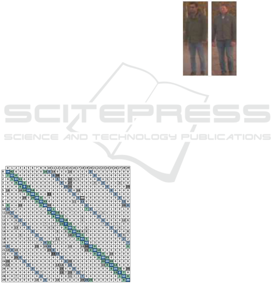
APPENDIX
Figure 8: Confusion matrices of the supervised (top) and
the cosine (bottom) approach.
VEHITS 2020 - 6th International Conference on Vehicle Technology and Intelligent Transport Systems
360
