
Accurate 3D Object Detection from Point Cloud Data using Bird’s Eye
View Representations
Nerea Aranjuelo
1,2
, Guus Engels
3
, David Montero
1,2
, Marcos Nieto
1
,
Ignacio Arganda-Carreras
2,4,5
, Luis Unzueta
1
and Oihana Otaegui
1
1
Vicomtech, Basque Research and Technology Alliance (BRTA), San Sebastian, Spain
2
University of the Basque Country (UPV/EHU), San Sebastian, Spain
3
AI In Motion (AIIM), Eindhoven, The Netherlands
4
Ikerbasque, Basque Foundation for Science, Bilbao, Spain
5
Donostia International Physics Center (DIPC), San Sebastian, Spain
Keywords:
Point Cloud, Object Detection, Deep Neural Networks, LiDAR.
Abstract:
In this paper, we show that accurate 3D object detection is possible using deep neural networks and a Bird’s
Eye View (BEV) representation of the LiDAR point clouds. Many recent approaches propose complex neural
network architectures to process directly the point cloud data. The good results obtained by these methods
have left behind the research of BEV-based approaches. However, BEV-based detectors can take advantage of
the advances in the 2D object detection field and need to handle much less data, which is important in real-
time automotive applications. We propose a two-stage object detection deep neural network, which takes BEV
representations as input and validate it in the KITTI BEV benchmark, outperforming state-of-the-art methods.
In addition, we show how additional information can be added to our model to improve the accuracy of the
smallest and most challenging object classes. This information can come from the same point cloud or an
additional sensor’s data, such as the camera.
1 INTRODUCTION
Over the last years, object detection has attracted
much research attention in the computer vision field.
Different methods have emerged related to an increas-
ingly improved 2D object detection thanks to the ad-
vances in Deep Learning (DL) (Ren et al., 2015; Du
et al., 2020). However, many applications, such as ad-
vanced driving, need 3D object detection. 3D object
detection is a less mature problem compared to 2D
detection, but it is fundamental for perception sys-
tems in the automotive field. In the last years, the
rapid progress of deep neural networks (DNNs) and
the emergence of the LiDAR sensor for the automo-
tive, have promoted the research in 3D object detec-
tion from LiDAR data.
Data captured by the LiDAR sensor is used to
construct 3D point clouds, which can be interpreted
as sparse 3D reconstructions of the ego-vehicle sur-
roundings, as shown in Figure 1. Different data repre-
sentations have been explored to adequate these point
clouds for the object detection algorithms. The first
methods mainly focused on converting the point cloud
to image-like representations, most of the time Bird’s
Eye View (BEV) or front view representations (Zhou
et al., 2019b). Recently, methods that process the
3D point clouds directly have gained popularity (Yan
et al., 2018; Lang et al., 2019). These methods show
good results and have replaced most of the previous
image-based models in the 3D object detection bench-
marks, such as the KITTI benchmark (Geiger et al.,
2012).
In this work, we show that accurate 3D object de-
tection can be done using the BEV representation of
LiDAR point clouds. We design a two-stage object
detection network architecture, which processes BEV
images and predicts robust 3D object detections. We
validate our approach in the KITTI benchmark and
show state-of-the-art results with no need for complex
detection pipelines. Our work proves that BEV-based
detection research should not be left behind. BEV-
based object detection has advantages compared to
direct point cloud processing. For example, it relies
on a light-weight representation of the scene. A Velo-
246
Aranjuelo, N., Engels, G., Montero, D., Nieto, M., Arganda-Carreras, I., Unzueta, L. and Otaegui, O.
Accurate 3D Object Detection from Point Cloud Data using Bird’s Eye View Representations.
DOI: 10.5220/0010688400003063
In Proceedings of the 13th International Joint Conference on Computational Intelligence (IJCCI 2021), pages 246-253
ISBN: 978-989-758-534-0; ISSN: 2184-3236
Copyright © 2023 by SCITEPRESS – Science and Technology Publications, Lda. Under CC license (CC BY-NC-ND 4.0)

Figure 1: 3D point cloud generated using the data captured
by a LiDAR (example scan from the KITTI benchmark).
dyne HDL-64E generates a point cloud up to 2.2 mil-
lion points per second, but the BEV representation re-
duces this point cloud to a 3-channel image covering
the area of interest. This image could be easily shared
with other agents in a cooperative scenario, allows a
fast inference, and is less resource-demanding than
processing a 3D point cloud. Our results demonstrate
that these conveniences are not at odds with high de-
tection accuracy.
Our contribution is twofold:
• We propose an object detection neural network for
LiDAR data that achieves state-of-the-art accu-
racy in the KITTI BEV benchmark with a simple
and reproducible object detection pipeline based
on BEV representations.
• We show how different additional data can be
added to the point cloud BEV representation to
boost small objects’ accuracy using the proposed
architecture.
2 RELATED WORK
2.1 Point Cloud Representations for
Image-oriented Architectures
When 3D object detection using DNNs and the Li-
DAR started gaining attention, most of the focus was
still on 2D object detection for image data. Con-
sequently, many methods converted point clouds to
image-like data so that state-of-the-art detectors could
be used.
In the literature, we find two main ways to do
the conversion from point cloud to image. The first
way is using a front view image in a polar coordinate
representation, which is the native representation of
the LiDAR sensor. 3D points from the LiDAR data
are projected on a depth map to create a front view
image (Zhou et al., 2019b). The images produced
are similar to the images from a camera. These im-
ages have a dense pixel representation. Consequently,
there may be occlusions between the objects in the
image, and the objects’ size is related to the distance
to the sensor. Different works use the front view as
the only or as a complementary representation (Chen
et al., 2017).
The second approach is creating a BEV im-
age (Yang et al., 2018), which represents the point
cloud from a top view perspective. With this ap-
proach, there might be a big compression in the height
dimension. This could be a challenge for classes that
are difficult to see from a top view perspective (e.g.,
pedestrians) because most of their information is in
the height dimension. However, thanks to the top-
view perspective, objects are clearly separated and
there are no occlusions between them. Moreover, all
objects of a specific class are the same size, indepen-
dent of the distance to the sensor, as the object di-
mensions are proportional to the real ones. The BEV
representation has been the most used pre-processing
step for 3D object detection from the LiDAR data and
is used by many methods (Yang et al., 2018; Simon
et al., 2019).
DNNs are not limited to one of the described rep-
resentations and some methods combine the benefits
of both. Some of these networks do not only rely on
the LiDAR but they also add front camera data (Qi
et al., 2018).
2.2 Image-oriented Architectures for
Object Detection
Object detection DNN architectures are often divided
in two main categories. The first is a single-stage
approach like YOLO (Redmon and Farhadi, 2018)
where anchor boxes are directly related to output
boxes. Two-stage methods like Faster R-CNN (Ren
et al., 2015) first try to identify regions of interest
(ROIs) that are likely to hold an object and then, in the
second stage, fit the bounding more tightly around the
object and decide to which class the object belongs
to. Generally the single stage models are faster while
the two-stage methods are more accurate. Both cate-
gories are the base of most 3D object detection works
(Simon et al., 2019; Chen et al., 2017).
Accurate 3D Object Detection from Point Cloud Data using Bird’s Eye View Representations
247

Figure 2: Proposed 3D object detection pipeline from LiDAR point cloud data.
2.3 Point Cloud Processing
Architectures
Converting point clouds to images involves gener-
ating a representation based on engineered features.
Some recent architectures for 3D object detection pro-
pose to learn on the point cloud data directly without
the conversion to image-like data. One of the first
methods that applied this idea is VoxelNet (Zhou and
Tuzel, 2018). They use a VFE-layer to learn fea-
tures from all the raw points in a particular voxel.
PointNet (Qi et al., 2017) goes a step further and can
directly consume points without any voxelization or
pre-processing. Although the original paper is not ap-
plied to the KITTI benchmark, it is the foundation for
many other methods (Yan et al., 2018; Lang et al.,
2019; Zhou et al., 2020; Shi et al., 2018). Due to the
improved accuracy of these methods in benchmarks
such as KITTI, little attention is paid now to the devel-
opment of better BEV-based methods. Most state-of-
the-art networks are based on a VoxelNet or PointNet-
like approach. Handling directly the point cloud data
involves some extra challenges, such as the volume of
data to be processed in real-time or the unstructured
form of the data. BEV-based methods are left behind
without a clear answer to the following questions: is it
better to process point clouds directly? Is it possible
to achieve similar results with BEV-based methods?
In this work, we aim at answering these questions.
3 METHODS
We propose a DNN that takes as input the BEV rep-
resentation of a point cloud and outputs the 2D ori-
ented bounding boxes corresponding to the detected
objects. The heights of the 3D boxes are estimated
based on the highest point inside each box. The entire
pipeline is shown in Figure 2.
3.1 Point Cloud to BEV Representation
Our approach first converts the point clouds to BEV
images. Different works use varying configurations,
resolutions and amount of height channels for this
Figure 3: Point cloud conversion to BEV representation.
step. We opt for keeping the height of the highest
points in every voxel as in (Aranjuelo et al., 2020).
This process is shown in Figure 3.
We consider a resolution of 0.1m for discretiz-
ing the point cloud in a grid of columns from a
top-view perspective. We keep the height informa-
tion in 3 channels to have an RGB-like data struc-
ture. Each column is divided into three voxels. Each
voxel is of size 0.1m × 0.1m × 1m, which results in
a 700 × 700 × 3 image (we consider a maximum dis-
tance of 70m in the longitudinal direction and 35m in
both sides in the lateral direction). For every pixel,
there will be three voxels. From all the points in each
voxel, we only keep the highest point’s height infor-
mation and discard the rest. This process compresses
the data but leaves enough information to detect ob-
jects.
3.2 Baseline Architecture
We base our network on Faster R-CNN (Ren et al.,
2015) with a ResNet50 (He et al., 2016) backbone
with some modifications related to the BEV repre-
sentations used as the input data. The BEV images
used in our research contain small objects, which are
challenging for being detected. In addition, we want
to detect oriented bounding boxes, rather than axis-
aligned detections as done in (Ren et al., 2015). Next,
we describe the proposed changes.
Our first modification is using a Feature Pyramid
Network-like architecture (Lin et al., 2017) to detect
objects at the higher-resolution feature maps and not
just at the final output maps of the ResNet.
Secondly, we adjust the stride of the third ResNet
blocks from 2 to 1. This prevents the feature maps
from being downsampled too quickly, which would
NCTA 2021 - 13th International Conference on Neural Computation Theory and Applications
248

lose detailed spatial information.
Thirdly, we remove the last ResNet block since we
empirically found that it did not improve the results
and allows for faster processing. The features ex-
tracted in this block probably do not contribute much
because of the too large receptive field of the pixels at
this depth. The receptive field after the third ResNet
block for each output value is already 195 pixels of
the original BEV image, which corresponds with al-
most a 20m x 20m area when using a 0.1m resolu-
tion. Although the context can help to detect the ob-
jects and the effective receptive field is smaller than
the theoretical one (Luo et al., 2016), it seems to be
already a large enough region.
We also use custom anchor boxes. The size of a
car is consistent everywhere in the image because of
the relation between their real size and their represen-
tation in the BEV image. This allows designing an-
chor boxes that best fit cars, pedestrians, and cyclists.
In the second stage of the network, we use ROI-
Align (He et al., 2017) to get 14×14 candidate ROIs,
which are max pooled with a 2 × 2 kernel and fed
to three fully connected layers with 1024 parameters
each. After each layer, a ReLU activation function is
used.
Lastly, the output detection bounding boxes are
processed by the non-maximum suppression (NMS)
method (Ren et al., 2015), so that unwanted bounding
boxes are removed based on their classification score
and the overlap between the boxes. If the classifica-
tion scores of overlapping correct and incorrect boxes
are mistaken by the DNN, this may lead to poor re-
sults. To make these classification scores more robust
based on the LiDAR data peculiarities, we compute
the percentage of non-empty pixels of each candidate
box. The correctly oriented boxes are mostly the ones
with a higher density of points, so we add this value
to the classification score to help the NMS choose the
correct detections.
3.2.1 Bounding Box Regression
The original Faster R-CNN network regresses axis-
aligned bounding boxes (with no orientation). The
bounding box regression is done in two stages. The
first bounding box regression step is in the Region
Proposal Network (RPN). In addition, the network
does a second bounding box regression at the end
of the second stage. Both steps regress axis-aligned
bounding boxes, which are represented by the cen-
ter of the bounding box (x, y) and the dimensions of
the bounding box (h, w). For an accurate 3D detec-
tion we need to detect oriented bounding boxes, so an
additional parameter (theta) has to be added for re-
gressing the angle of the bounding box. We maintain
the axis-aligned regions’ regression in the RPN but
regress five parameters in the second stage, which in-
clude the orientation of the box. The oriented bound-
ing box parameters can be regressed individually with
a loss function like L1, L2, or smooth L1. The un-
derlying assumption is that regressing these param-
eters individually will lead to a global optimum for
the bounding box estimation. For axis-aligned boxes,
this seems to work, but for oriented bounding boxes
does not. Qian et al. (2019) show the conflicting inter-
est between the angle regression and the other regres-
sions. A way to solve this problem is to directly min-
imize the loss for what you are evaluating on, which
is the intersection over union (IoU) between ground
truth and estimated bounding boxes. We use the IoU
loss for the second stage (Zhou et al., 2019a).
3.2.2 Loss Function
Regarding the loss function, both network stages have
a regression loss and a classification loss. Conse-
quently, the total loss is a combination of four losses.
The first stage is the RPN and uses the same loss ob-
jectives as the original Faster R-CNN. Four regres-
sion parameters are optimized with a smooth L1 loss,
being (x, y) the center and (h, w) the dimensions of
the bounding box. Once the difference between the
ground truth parameter and the estimated one is com-
puted (d), the smooth L1 loss is used according to the
following Equation 1:
L1(d) =
(
0.5d
2
σ if |d| <
0.5
σ
|d| −
0.5
σ
otherwise
(1)
where σ is a tuning hyperparameter. We use σ = 3
for the RPN network and σ = 1 for the head network,
as in the Faster R-CNN implementation (Ren et al.,
2015). The RPN classification loss is binary cross-
entropy with foreground and background boxes. In
the second stage, we use a IoU regression loss with
five regression parameters instead of four (Zhou et al.,
2019a). For the classification we use a multi-class
cross-entropy loss.
4 NETWORK EXTENSIONS
One of the biggest challenges for the BEV-based ob-
ject detection methods is to distinguish the smallest
objects (e.g., pedestrians). When converting point
clouds to BEV images a compression takes place
where some data are lost. This is not a problem if
there is enough data left to accurately perform detec-
tion of the target objects. When looking at the BEV
images, this clearly seems to be the case of the cars.
Accurate 3D Object Detection from Point Cloud Data using Bird’s Eye View Representations
249
Many points are discarded but they still show a clear
structure which makes it possible to detect them. This
is not so clear for small classes such as the pedestri-
ans and the cyclists. The top view perspective only
covers a small area of these objects. This might be al-
leviated with additional data that helps to distinguish
these objects from others. For this reason, we test two
network extensions. The first one uses data already
provided in the BEV image and the second one incor-
porates external data.
Each point in a LiDAR point cloud is represented
by its 3D coordinates and its reflectance values. These
values are related to the object class it represents and
can provide meaningful information. Even if some
of the values are stored in the BEV image, the spe-
cific pixel values are often lost along the network’s
operations (Engels et al., 2020). The detectors conse-
quently rely on the shape patterns in the BEV image
more than on the extra information provided by the
specific values. In order to test if these data could
complement the patterns learnt by the network, we
add a skip connection from the input BEV map to the
head network. This connection adds the raw values to
the data received in the head network (feature maps
of the candidate ROIs from the RPN) so that we guar-
antee that the values do not get discarded in the back-
bone and they can be used in the second stage of the
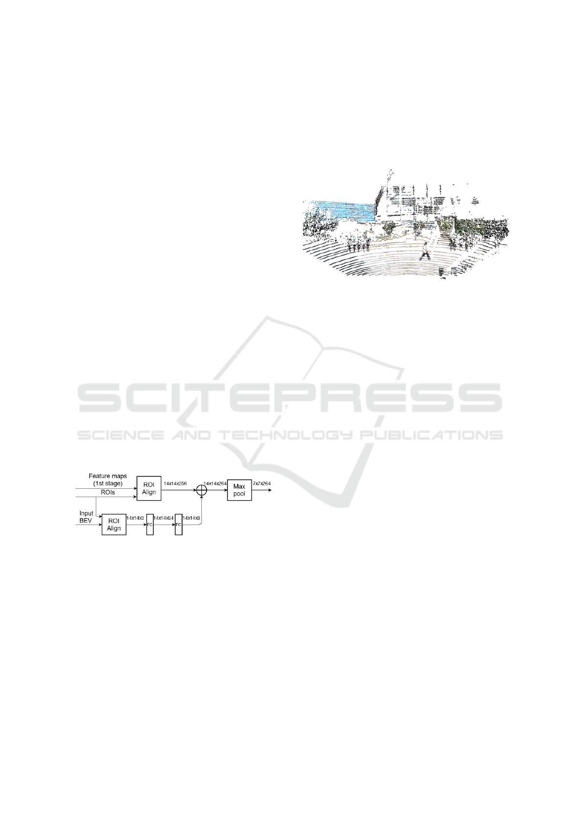
network. In addition, we add two fully connected lay-
ers to the input values before concatenating them to
the input data of the head network. These layers al-
low the network to learn a better fusion mechanism
from the two feature spaces. Figure 4 shows the fu-
sion scheme.
Figure 4: Fusion scheme to add information to the head
network from a BEV image.
Based on the same fusion scheme, we could add
information from a different BEV image instead of
the heights-based one we use as input to the network.
For instance, we can add data related to another sen-
sor, such as the camera. The camera captures infor-
mation about the textures and appearances of the ob-
jects. The information provided by the camera pixel
values about the object appearances is complimentary
to the data from the LiDAR and might help in gaining
robustness. To test this, we project the camera im-
age pixel values from the camera to the point cloud.
An example of the resulting point cloud is shown in
Figure 5. Next, we compute the BEV representation
which contains in each cell the pixel color informa-
tion instead of the height. Figure 6 shows an example
of this kind of BEV. The new BEV image is added to
the head network with the same fusion mechanism as
with the heights-based BEV image (Figure 4).
Figure 5: A LiDAR scan of the KITTI benchmark to which
its corresponding camera image RGB values are projected.
5 NETWORK OPTIMIZATION
The use of BEV images for 3D object detection re-
duces the amount of data to be handled. This trans-
lates into less processing time and makes the ap-
proach suitable for real-time applications or collab-
orative environments. The Faster R-CNN network is
more accurate than most single-stage object detection
architectures but also slower. Consequently, to make
the inference faster without reducing the architecture
complexity, we optimize the model after its training.
The number of proposals generated in the first net-
work stage varies in every image. However, the input
batch of the second stage remains fixed. If the num-
ber of generated proposals is smaller than the batch
number, the missing proposals need to be simulated
with empty ones. To avoid this processing, we di-
vide the network into two parts which correspond to
each stage and are treated as two independent net-
works running asynchronously. Thus, the first net-
work processes batches of N images and generates a
different number of proposals for each image, which
are processed together in one batch by the second net-
work. This way, the batch of the second network is
optimized for the total number of proposals.
Using a dynamic batch for the second network
may lead to time overheads, as the network needs
to be re-adapted for the new size. To avoid this,
the proposals are grouped together in batches of a
fixed size M and fed asynchronously to the network.
Once the proposals are classified, they are returned
again to their original batches according to the image
they belong to. We optimize the models with Ten-
sorRT (NVIDIA, 2021).
NCTA 2021 - 13th International Conference on Neural Computation Theory and Applications
250

Figure 6: A BEV image which contains the projected image
pixels color information instead of the heights of the points.
6 EXPERIMENTS
We test our approach on the KITTI dataset, which
has 7, 158 training samples. We use a 50/25/25 split
for training/validation/test sets. We convert the point
clouds to 700 × 700 × 3 images with a 0.1m resolu-
tion. Only the annotated area is considered, which
corresponds to the field of view of the camera. We
evaluate the network on the three classes of the bench-
mark but we train two separate networks, one for cars
and another for pedestrians and cyclists. For each net-
work, we train and evaluate three variants: the base-
line model, the baseline with the fusion of the input
BEV in the head network, and the same model but
with the fusion of the RGB data-based BEV. The car
class has by far the most objects, which is the rea-
son to train it apart. Otherwise, the network would be
very biased in favor of this class. The KITTI results
are evaluated by calculating average precision (AP)
for three difficulty categories (easy, moderate, hard)
for every class. We consider a x, y, z range of [(0, 70),
(-35, 35), (0, 3)] meters respectively for the car class
and [(-35, 35), (-35, 35), (0, 3)] meters for pedestri-
ans and cyclists. As proposed in the benchmark, we
use an IoU threshold of 0.7 for the cars, and 0.5 for
pedestrians and cyclists.
Regarding the training, our loss function is opti-
mized with stochastic gradient descent with a momen-
tum of 0.9. An initial learning rate of 0.003 is used
with decay steps at 35 and 42 epochs, with a factor of
0.1. The total network is trained for 70 epochs with a
batch size of 1 and a mini-batch size of 256. The mini-
batch corresponds to the number of region proposals
which are fed to the second stage. Weight decay is set
at 0.0001. The entire baseline model has 19M learn-
able parameters. The backbone is initialized with pre-
trained weights from ImageNet, whereas the head net-
work is trained from scratch. All tests are done on a
single Nvidia Tesla V100 GPU. All other hyperpa-
rameters are the same as used for the Faster R-CNN.
7 RESULTS AND DISCUSSION
Table 1 shows the AP obtained by our method com-
pared to other state-of-the-art approaches for car,
pedestrian and cyclist classes. In the same way as
in (Simon et al., 2019), we validate our results on
our splitted validation dataset, whereas the others are
validated on the official KITTI test set. Our mod-
els outperform most of the works with only LiDAR
data for the three classes and difficulties. Our pro-
posed CNN architecture achieves a higher AP than
other BEV-based pipelines, such as (Yang et al., 2018)
and (Simon et al., 2019). These models mainly dif-
fer in the proposed backbone architecture and the re-
gression loss. In addition, our work also surpasses
the approaches which process raw point clouds, such
as (Yan et al., 2018) and (Lang et al., 2019). Only the
method in (Zhou et al., 2020) presents a slightly bet-
ter accuracy for cars in the hard category. This shows
that using a BEV-based approach is not a limitation
for obtaining a high detection accuracy.
Regarding the network extension tests, no im-
provement is obtained for the car class. This may be
because the cars had already enough points and in-
formation for being accurately detected in the BEV
image. This is not the case of smaller objects such as
pedestrians and cyclists. Adding the skip connection
with the input values to the head network boosts the
accuracy of the cyclist class. Regarding the addition
of the camera-based BEV image, it increments the ac-
curacy of the pedestrian and cyclist detections. When
comparing this network to another multimodal ap-
proach like (Qi et al., 2018), we observe that the accu-
racy obtained by Frustum PointNets is higher for the
pedestrian class, but not for the cars and the cyclists.
This may happen because of the feature space where
the detections are estimated. Frustum PointNets de-
tect the object proposals on the RGB image and then,
computing a 3D viewing frustum, they predict the fi-
nal 3D box on the point cloud. Therefore, the accu-
racy is closely related to the 2D detector for the RGB
image. This differs from our approach, which projects
the RGB values to the point cloud instead of detecting
the objects in the RGB image. For small classes in the
BEV representation, the camera detections seem to be
more reliable, even if the projected information boosts
the BEV-based detection accuracy.
Figure 7 shows some qualitative results of the
baseline model on the BEV images. The left image
corresponds to the model trained on cars, whereas the
right image shows the detections from the pedestrian
and cyclist model (only pedestrians are present in the
image). The mean inference time per scan (entire
pipeline) is 30 ms. Figure 8 shows the same detec-
Accurate 3D Object Detection from Point Cloud Data using Bird’s Eye View Representations
251
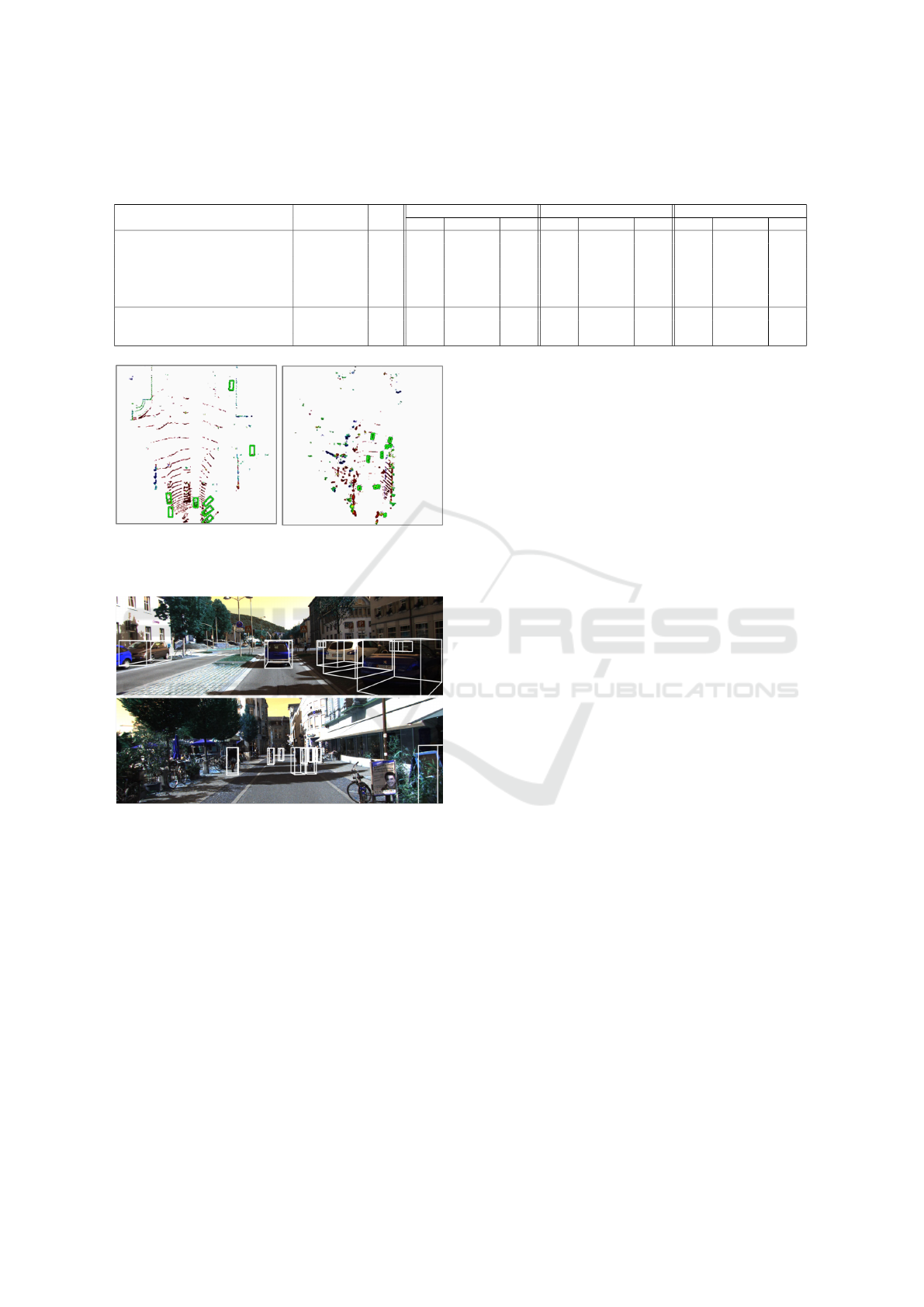
Table 1: Our proposed approach compared to other state-of-the-art methods on our KITTI val set based on the AP. Note that
our work and (Simon et al., 2019) are validated on our split validation dataset, whereas all others are validated on the official
KITTI test set.
Method Modality BEV
Car Pedestrian Cyclist
Easy Moderate Hard Easy Moderate Hard Easy Moderate Hard
PIXOR (Yang et al., 2018) LiDAR Yes 81.70 77.05 72.95 N/A N/A N/A N/A N/A N/A
Complex-YOLO (Simon et al., 2019) LiDAR Yes 85.89 77.40 77.33 46.08 45.90 44.20 72.37 63.36 60.27
PointPillars (Lang et al., 2019) LiDAR No 88.35 86.10 79.83 58.66 50.23 47.19 79.14 62.25 56.0
SECOND (Yan et al., 2018) LiDAR No 88.07 79.37 77.95 55.10 46.27 44.76 73.67 56.04 48.78
Joint 3D (Zhou et al., 2020) LiDAR No 90.23 87.53 86.45 N/A N/A N/A N/A N/A N/A
F-PointNets (Qi et al., 2018) RGB+LiDAR No 88.16 84.02 76.44 72.38 66.39 59.57 81.82 60.03 56.32
Baseline LiDAR Yes 97.3 89.6 85.0 54.1 52.5 51.0 73.2 60.7 58.7
Baseline + input BEV LiDAR Yes 93.7 88.7 84.4 52.9 51.7 49.1 80.4 66.6 64.2
Baseline + camera-based BEV RGB+LiDAR Yes 94.6 87.1 83.3 56.1 54.0 50.7 82.6 73.1 70.5
Figure 7: Qualitative results on our KITTI val set. Detec-
tions are shown on the BEV representation for the car class
(left) and the pedestrian class (right).
Figure 8: Qualitative results on our KITTI val set. Detec-
tions are shown on the BEV representation (left) and pro-
jected to the camera image (right).
tions projected to the camera images for better visual-
ization of the results.
The optimization applied to the trained DNNs al-
lows scaling the detection task to process different
BEV images at the same time. The batch-oriented op-
timization may be interesting for processing the data
from the different LiDARs of a vehicle or for an au-
tomotive ground truth annotation application that re-
quires handling batches of scans. Compared to a 3D
CNN, the computational cost of a BEV-based CNN is
lower. The computational complexity of a 3D CNN
grows cubically with the voxel resolution (Yan et al.,
2018). In addition, the BEV representation reduces
the target raw point cloud (up to millions of points) to
a 3-channel image covering the area of interest and
filtering many points that are not significant. The
biggest challenge for BEV-based methods is the de-
tection of the objects covering a small area in the BEV
image.
Given the advantages of a BEV-based method and
the accuracy achieved by the proposed DNNs, we
conclude that methods processing raw point clouds
should not be led to abandon or replace the BEV-
based detection research.
8 CONCLUSIONS
In this paper, we propose a 3D object detection
pipeline based on a two-stage neural network archi-
tecture for detecting objects from LiDAR point cloud
data. Our method relies on BEV representations and
does not need to process entire raw point clouds. We
propose two network extensions for boosting the ac-
curacy of the most challenging object classes, based
on adding BEV data to the head network. We evaluate
our method on the KITTI BEV benchmark and show
that it achieves state-of-the-art results. It surpasses
recent methods based both on BEV images or raw
point clouds. Moreover, our results show that BEV-
based detection research should not be replaced with
complex point cloud-based detectors. Using a BEV
representation does not limit the detection accuracy
and provides advantages such as the light-weight rep-
resentation of the scene, which is suitable for being
shared in a cooperative scenario or for a fast infer-
ence.
Future work includes improving the model to han-
dle different classes which have different sizes in the
BEV images (e.g., trucks, pedestrians) and are mostly
unbalanced in the public datasets. We also plan to val-
idate our approach in benchmarks with different types
of LiDAR sensors.
NCTA 2021 - 13th International Conference on Neural Computation Theory and Applications
252

ACKNOWLEDGEMENTS
This work has received funding from Basque Govern-
ment under project AUTOLIB of the program ELKA-
RTEK 2019.
REFERENCES
Aranjuelo, N., Engels, G., Unzueta, L., Arganda-Carreras,
I., Nieto, M., and Otaegui, O. (2020). Robust 3d ob-
ject detection from lidar point cloud data with spatial
information aggregation. In International Workshop
on Soft Computing Models in Industrial and Environ-
mental Applications, pages 813–823. Springer.
Chen, X., Ma, H., Wan, J., Li, B., and Xia, T. (2017). Multi-
view 3d object detection network for autonomous
driving. In Proceedings of the IEEE Conference
on Computer Vision and Pattern Recognition, pages
1907–1915.
Du, X., Lin, T.-Y., Jin, P., Ghiasi, G., Tan, M., Cui, Y., Le,
Q. V., and Song, X. (2020). SpineNet: Learning scale-
permuted backbone for recognition and localization.
In Proceedings of the IEEE/CVF conference on com-
puter vision and pattern recognition, pages 11592–
11601.
Engels, G., Aranjuelo, N., Arganda-Carreras, I., Nieto, M.,
and Otaegui, O. (2020). 3d object detection from li-
dar data using distance dependent feature extraction.
arXiv preprint arXiv:2003.00888.
Geiger, A., Lenz, P., and Urtasun, R. (2012). Are we ready
for autonomous driving? the KITTI vision benchmark
suite. In 2012 IEEE conference on computer vision
and pattern recognition, pages 3354–3361. IEEE.
He, K., Gkioxari, G., Doll
´
ar, P., and Girshick, R. (2017).
Mask r-cnn. In Proceedings of the IEEE international
conference on computer vision, pages 2961–2969.
He, K., Zhang, X., Ren, S., and Sun, J. (2016). Deep resid-
ual learning for image recognition. In Proceedings of
the IEEE conference on computer vision and pattern
recognition, pages 770–778.
Lang, A. H., Vora, S., Caesar, H., Zhou, L., Yang, J., and
Beijbom, O. (2019). Pointpillars: Fast encoders for
object detection from point clouds. In Proceedings
of the IEEE/CVF Conference on Computer Vision and
Pattern Recognition, pages 12697–12705.
Lin, T.-Y., Doll
´
ar, P., Girshick, R., He, K., Hariharan, B.,
and Belongie, S. (2017). Feature pyramid networks
for object detection. In Proceedings of the IEEE con-
ference on computer vision and pattern recognition,
pages 2117–2125.
Luo, W., Li, Y., Urtasun, R., and Zemel, R. (2016). Under-
standing the effective receptive field in deep convo-
lutional neural networks. In Proceedings of the 30th
International Conference on Neural Information Pro-
cessing Systems, pages 4905–4913.
NVIDIA (2021). TensorRT: A platform for high-
performance deep learning inference. https://
developer.nvidia.com/tensorrt. Accessed: 07.01.2021.
Qi, C. R., Liu, W., Wu, C., Su, H., and Guibas, L. J. (2018).
Frustum pointnets for 3d object detection from rgb-d
data. In Proceedings of the IEEE conference on com-
puter vision and pattern recognition, pages 918–927.
Qi, C. R., Su, H., Mo, K., and Guibas, L. J. (2017). Point-
net: Deep learning on point sets for 3d classification
and segmentation. In Proceedings of the IEEE con-
ference on computer vision and pattern recognition,
pages 652–660.
Qian, W., Yang, X., Peng, S., Guo, Y., and Yan, J. (2019).
Learning modulated loss for rotated object detection.
arXiv preprint arXiv:1911.08299.
Redmon, J. and Farhadi, A. (2018). Yolov3: An incremental
improvement. arXiv preprint arXiv:1804.02767.
Ren, S., He, K., Girshick, R., and Sun, J. (2015). Faster R-
CNN: Towards real-time object detection with region
proposal networks. Advances in neural information
processing systems, 28:91–99.
Shi, S., Wang, X., and Li, H. (2018). PointRCNN: 3d object
proposal generation and detection from point cloud.
CoRR, abs/1812.04244.
Simon, M., Amende, K., Kraus, A., Honer, J., Samann,
T., Kaulbersch, H., Milz, S., and Michael Gross, H.
(2019). Complexer-yolo: Real-time 3d object detec-
tion and tracking on semantic point clouds. In Pro-
ceedings of the IEEE/CVF Conference on Computer
Vision and Pattern Recognition Workshops, pages 0–
0.
Yan, Y., Mao, Y., and Li, B. (2018). Second:
Sparsely embedded convolutional detection. Sensors,
18(10):3337.
Yang, B., Luo, W., and Urtasun, R. (2018). Pixor: Real-time
3d object detection from point clouds. In Proceedings
of the IEEE conference on Computer Vision and Pat-
tern Recognition, pages 7652–7660.
Zhou, D., Fang, J., Song, X., Guan, C., Yin, J., Dai, Y., and
Yang, R. (2019a). Iou loss for 2d/3d object detection.
In 2019 International Conference on 3D Vision (3DV),
pages 85–94. IEEE.
Zhou, D., Fang, J., Song, X., Liu, L., Yin, J., Dai, Y., Li, H.,
and Yang, R. (2020). Joint 3d instance segmentation
and object detection for autonomous driving. In Pro-
ceedings of the IEEE/CVF Conference on Computer
Vision and Pattern Recognition, pages 1839–1849.
Zhou, J., Tan, X., Shao, Z., and Ma, L. (2019b). FVnet:
3d front-view proposal generation for real-time ob-
ject detection from point clouds. In 2019 12th In-
ternational Congress on Image and Signal Process-
ing, BioMedical Engineering and Informatics (CISP-
BMEI), pages 1–8. IEEE.
Zhou, Y. and Tuzel, O. (2018). Voxelnet: End-to-end learn-
ing for point cloud based 3d object detection. In Pro-
ceedings of the IEEE conference on computer vision
and pattern recognition, pages 4490–4499.
Accurate 3D Object Detection from Point Cloud Data using Bird’s Eye View Representations
253
