Machine Learning for Drone Conflict Prediction: Simulation Results

Brian Hilburn

Center for Human Performance Research, Amsterdam, The Netherlands

Keywords: Machine Learning, Drone, Urban Air Mobility.

Abstract: Introducing drones into urban airspace poses several air traffic management (ATM) challenges. Among these

is how to monitor and de-conflict (potentially high-density / low predictability) drone traffic. This task might

exceed the capabilities of the current (human-based) air traffic control system. One potential solution lies in

the use of Machine Learning (ML) to predict drone conflicts. This study explored via low-fidelity offline

simulations the potential benefits of ML for drone conflict prediction, specifically: how well can a simple ML

model predict on the basis of instantaneous traffic pattern snapshot, whether that pattern will result in an

eventual airspace conflict? Secondly, how is model performance impacted by such parameters as traffic level,

traffic predictability, and ‘look-ahead’ time of the model?

Using a deep learning neural network approach, this study experimentally manipulated traffic load, traffic

predictability, and look-ahead time. Using limited trajectory data (aircraft state) and a limited neural network

architecture, results demonstrated (especially with structured traffic) large potential ML benefits on airspace

conflict prediction. Binary classification accuracy generally exceeded 90%, and error under the most

demanding scenarios tended toward false positive (i.e. incorrectly predicting a conflict). The current work is

abstracted from Hilburn (2020), which provides further detail.

1 INTRODUCTION

The possible introduction of drone traffic into urban

airspace has many in the air traffic management

(ATM) community wondering how to accommodate

such a fundamentally new type of aircraft, whose

potential numbers and unpredictability might

overwhelm current human-based methods for

managing air traffic (Duvall et al., 2019; European

Union, 2016). One possible solution lies in the use of

Machine Learning (ML) techniques for predicting

(and possibly resolving) drone conflicts in high

density airspace.

The aim of this research was not to develop an

optimised ML model per se, but to experimentally

explore via low-fidelity offline simulations the

potential benefits of ML for drone conflict prediction,

specifically: how well can a simple ML model predict

on the basis of instantaneous traffic pattern snapshot,

whether that pattern will result in an eventual airspace

conflict (defined as entry into a stationary prohibited

zone)?

https://orcid.org/0000-0001-8585-5902

Secondly, how is model performance impacted by

such parameters as traffic level, traffic predictability,

and ‘look-ahead’ time of the model?

2 METHOD

2.1 Airspace and Traffic Assumptions

This effort started from several assumptions. First

was the focus on the ‘edge case,’ or worst-case

scenario. If ML were able to predict conflicts under

the most challenging possible assumptions, real

world results would likely be better. For reasons of

this analysis, traffic assumptions therefore included

the following (TERRA, 2019):

• Urban Air Mobility (UAM) scenario —

envisions short flight times, and frequent

trajectory changes;

• High traffic density—this is implicit in

predicted future urban drone scenarios, but we

intended to push the limits of traffic level;

Hilburn, B.

Machine Learning for Drone Conﬂict Prediction: Simulation Results.

DOI: 10.5220/0011963700003622

In Proceedings of the 1st International Conference on Cognitive Aircraft Systems (ICCAS 2022), pages 77-82

ISBN: 978-989-758-657-6

 2023 by SCITEPRESS – Science and Technology Publications, Lda. Under CC license (CC BY-NC-ND 4.0)

• Lack of intent information—no flight plan

information (regarding filed destination,

speed, altitude, heading changes, etc) would

be available. Instead, only the minimal

(instantaneous) state information would be

provided;

• Random drone movements—ML conflict

prediction would be trivial if all drone

movements were completely predictable. In

reality, VLL drone operations will have a fair

amount of structure and determinism.

However, we intentionally introduced a high

level of randomness in drone movements,

again to test the worst case scenario for ML;

• Prohibited airspace— was represented as

static no-go regions (e.g, around security

sensitive areas). This analysis included a

single, static “no drone zone,” and conflicts

were defined as penetrations of this zone.

2.2 Methodological Assumptions

This effort set out to test ML conflict prediction using

the most challenged methods. Specifically, this meant

that whatever ML model we used, must have no

ability to look either forward or backward in time, nor

make use of any other information beyond the simple

instantaneous state of each drone. For research

purposes, the conflict prediction problem was

simplified to one of pattern recognition. We used a

supervised learning approach, and in particular a

fairly limited architecture: the standard deep learning

(i.e., multi hidden layer) artificial neural net. Whereas

enhancements to the neural net approach (including

RNN, CNN, and LSTM enhancements) would be

expected to show better time series processing and

thus better classification performance, we set out to

use a simpler neural net architecture, to establish

baseline worst case model performance. Moreover,

we set out to train different models (36 in all) so that

model performance could be compared

experimentally, to assess the impact of traffic level,

traffic randomness, and look-ahead window range, on

ML conflict prediction performance.

2.3 Test Scenarios and Traffic Samples

The urban drone environment was represented by a

20 x 20 grid of 400 total cells. Each cell was either

occupied or empty. Developmental testing

established the number and size of restricted areas, so

as to produce a reasonable number of Prohibited Zone

(PZ) incursions. It was decided to use a single,

stationary PZ, as shown in 1. One simplifying

assumption was that altitude was disregarded, and

drone movements were only considered in two

dimensions (the PZ was assumed to be from the

surface upward). Second, there were no speed

differences between drones. Finally, conflicts were

only defined as airspace incursions into the PZ, not as

losses of separation between drones (drones were

assumed to maintain vertical separation).

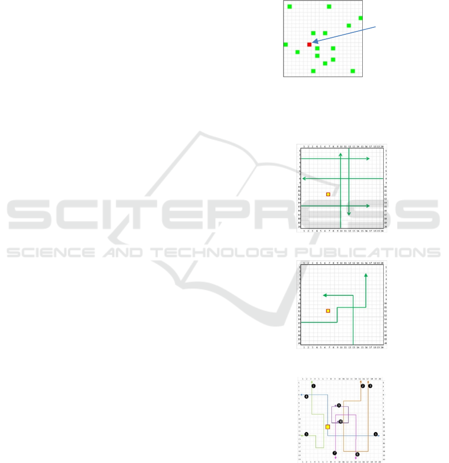
Figure 1: Snapshot, traffic sample of 16 birthed drones

(note PZ).

Traffic samples were built from three different kinds

of drone routes, as shown in Figure 2.

(a) Through-routes.

(b) TCP-routes.

Figure 2: The three types of drone routes.

Notice that drones could only fly on cardinal

headings (North, South, East, or West). Through-

ICCAS 2022 - International Conference on Cognitive Aircraft Systems

routes transited the sector without any heading

change. TCP-routes (i.e. Trajectory Change Point

routes) added probabilistic heading changes to

through-routes. After a random interval of 3-6 steps,

TCP-route drones would either continue straight

ahead, or make a 90° left/right heading change. The

random TCP function was nominally weighted to

50% no heading change (i.e. continue straight ahead),

25% left turn, and 25% right turn. Finally, the ten

possible Bus-routes (5 routes, flown in either

direction) were pre-defined TCP trajectories. Bus-

route drones all entered the sector after sample start

time, except for bus-routes 9 and 10 (which flew a

square pattern in the centre of the sector, and were

birthed already on their route).

As discussed later, analysis compared “random”

and “structured” route conditions, as an experimental

manipulation. The random condition used TCP-

routes exclusively. The structured condition used a

random combination of through-routes and bus-

routes.

Each traffic sample consisted of 40 time steps.

First appearance of each drone was randomly timed

to occur between steps 1 and 15. Each drone

maintained current heading by advancing one cell per

time step (no hovering). This meant that a through-

route drone would transit the sector in 20 steps. Each

traffic sample also consisted of 4, 8, or 16 birthed

drones (this was also an experimental manipulation,

as described later). Because birth time was

randomized, the actual number of instantaneous in-

sector drones could vary.

Analysis used a 3x2x2 experimental design and

varied the following factors:

• Aircraft count (4 vs 8 vs 16)— the total

number of birthed aircraft;

• Look-ahead time (Low vs High)— Snapshot

time, in number of steps before conflict;

• Traffic structure (Low vs High)—

Randomised vs semi-structured traffic flows.

2.4 Neural Network Design

Neural network modelling was done in

NeuralDesigner v2.9, a machine learning toolbox for

predictive analytics and data mining, built on the

Open NN library. Modelling used a 400.3.1

architecture (i.e., 400 input nodes, a single hidden

layer of 3 nodes, and a single binary output node),

with standard feedforward and back propagation

mechanisms, and a logistic activation function. Each

of the 400 total cells was represented as an input node

to the network. Each input node was simply coded on

the basis of occupation, i.e. a given cell was either

occupied (1) or empty (0). The output node of the

ANN was simply whether the traffic pattern evolved

into an eventual conflict (0/1). Maximum training

iterations with each batch was set to 1000.

2.5 Procedures

The overall flow of the traffic generation, pre-

processing, and ANN modelling process is shown in

Figure 3. Using a traffic generation tool, preliminary

batches of 5000 traffic samples each were created.

Separate batches were created for each combination

of aircraft count and structure level. For each batch,

samples were then automatically processed to

identify conflict versus non-conflict outcomes,

extract multiple look-ahead snapshots (for 1-6 steps)

from conflict samples, and extract matching yoked

snapshots from non-conflict samples. Target outputs

were then labelled, and sample groups were fused into

a final batch file. This batch file was then randomly

split 60/40 into training and testing sub batch files.

After training each of the 36 networks with its

appropriate training sub batch file, each network was

tested on its ability to classify the corresponding test

sub batch file.

Figure 3: Overview, traffic creation and model testing

procedure.

3 RESULTS

3.1 Binary Classification Accuracy

The simplest performance measure is classification

accuracy. That is, what percentage of samples was

correctly classified as either conflict or no conflict?

The ANN models each had a simple binary output:

either an eventual conflict was predicted, or was not.

This is a classic example of a binary classification

task, which is characterized by two ‘states of the

world’ and two possible predicted states. A binary

classification table, as shown in Figure 4, allows us to

identify four outcomes: True Positive (TP), True

Negative (TN), False Positive (FP), and False

Negative (FN). According to Signal Detection Theory

Machine Learning for Drone Conﬂict Prediction: Simulation Results

(Green & Swets, 1966), these outcomes are referred

to, respectively, as: Hits, Correct Rejections, False

Alarms, and Misses.

Figure 4: Binary classification outcomes.

These four classification outcomes allow us to define

the following rates:

• Accuracy— the rate of proper classification,

defined as: ACC = [TP+TN] /

[TP+FN+TN+FP]

• Error Rate = 1-ACC = [FN+FP] /

[TP+FN+TN+FP]

• True Positive Rate (aka sensitivity) = TP /

[TP+FN]

• True Negative Rate (aka specificity) = TN /

[TN+FP]

For structured traffic, there seemed to be a ceiling

effect on classification performance. Classification

accuracy approached optimum (falling no lower than

.948) regardless of traffic or look-ahead time. This

means that, with structured traffic, the ANN model

was able to predict almost perfectly which traffic

samples would result in conflict. This was not

surprising. As discussed earlier, under structured

traffic the majority (84%) of drones would be

predictable by the second step after sector entry. By

step 3, the only uncertainty would be whether the

other 16% were on through-routes or bus-routes.

Random traffic, however, showed some variations

in model performance. Classification performance

with random traffic was still impressively high,

ranging from .72 to .98, and generally well above

chance levels. However, under random traffic we

began to see ML performance declines with both

look-ahead time and traffic count (classification

performance worsened with each), and a trend toward

a three-way interaction between traffic, structure, and

look-ahead.

Figure 5 shows the effect of both look-ahead and

aircraft count, on overall classification accuracy. Data

are somewhat collapsed in this view. Look-ahead (1-

6) is binary split into Low (1-3) and High (4-6).

Aircraft count includes only the extremes of 4 and 16.

Besides a main effect of both look-ahead (longer

look-ahead worsened performance) and aircraft count

(higher count worsened performance), there is a slight

trend toward a look-ahead x aircraft count interaction.

Notice the interaction trend, whereby longer look-

ahead had a greater cost under high traffic.

Figure 5: Effect of aircraft count and look-ahead on overall

classification performance, random traffic only.

3.2 Sensitivity and Specificity

For a finer-grained view, see the three panels of

Figure 6. These present classification performance

under random traffic, for low, medium, and high

aircraft count (from left to right panel). Each panel

also shows the impact of look-ahead, from 1-6 steps.

Figure 6: Classification performance, sensitivity, and

specificity, for random traffic (low to high, top to bottom).

ICCAS 2022 - International Conference on Cognitive Aircraft Systems

Notice that the pattern of Sensitivity (the TPR)

and Specificity (TNR) vary by aircraft count.

Basically, ML overall performance worsened with

look-ahead time, but the underlying patterns (TPR,

TNR) differed by aircraft count. For low traffic,

Sensitivity fell disproportionately (i.e., the model

tended toward FN rather than FP). For high traffic,

Specificity fell (the system tended toward FP rather

than FN). At the highest level, this interaction trend

suggests that the ANN model tended to

disproportionately false positive under the most

demanding traffic samples.

3.3 The Extreme Scenario

To test one final, and even more challenging case,

we generated traffic and trained / tested an ANN

model, using random traffic, 24 aircraft, and a look-

ahead of 6 (see Figure ).

Figure 7: The extreme scenario: 24 drones, random traffic,

and a six-step look-ahead.

Classification accuracy remained surprisingly high in

this condition (in fact, slightly above the 16 drone

sample). Also, this extreme scenario extended the

trend toward Specificity decrement seen in the three

panels of Figure 6.

Table 1: Results summary, binary classification

performance, extreme scenario.

Classification accuracy 0.739

Error rate 0.261

Sensitivity (TP) 0.705

Specificity (TN) 0.758

False Positive Rate (FP) 0.242

False Negative Rate (FN) 0.295

3.4 Summary of Results

In terms of conflict prediction performance, results

from our ML model can be summarized as follows:

• With structured traffic, overall model

performance was nearly perfect;

• With structured traffic, no effect of traffic

count nor look-ahead could be found;

• For random traffic, the model still performed

quite well;

• For random traffic, traffic count and (more so)

look-ahead had a clear impact on overall

classification accuracy;

• This look-ahead effect on accuracy revealed

subtle differences in other parameters. For low

traffic, Sensitivity (TP rate) declined more

than did Specificity (TN rate). For high traffic,

this was reversed, In other words, longer look-

ahead worsened overall classification

performance, but low traffic was biased

toward false negatives, and high traffic was

biased toward false positives;

• Even under the most challenging conditions

(random, high traffic, long look-ahead), ML

classification accuracy was still fairly high

(76.5%);

• Even with random traffic, classification

performance was generally well above

guessing level, far better than chance;

• The ANN approach continued to show robust

classification performance, even when

presented an extreme case of 24 drones,

random traffic, and long look-ahead.

4 CONCLUSIONS

Even with minimal data (i.e., nothing more than

instantaneous traffic snapshot), and a limited neural

network architecture (without any explicit time series

processing capability), neural network modelling

demonstrated potential benefits in predicting and

classifying drone trajectories in the urban

environment. We would expect ML methods, once

deployed, to show even better performance, for two

main reasons.

First, and as noted elsewhere, advanced ML

methods exist that can make better use of memory,

time series processing, time delays, and memory

erase functions. Static ANNs, which are limited in

their ability to handle time series data, have clear

limitations in predicting dynamic air traffic patterns.

Related ML methods such as recurrent neural

Machine Learning for Drone Conﬂict Prediction: Simulation Results

networks, convolutional neural networks, time delay

neural networks, and long short term memory would

all likely show better predictive performance.

Second, ML would presumably perform better

with meaningful real world data, rather than

stochastically generated flights. The neural network

approach (as with all ML methods) assumes that there

are some underlying patterns in the data which the

network can uncover. However, the pattern and

structure in our generated traffic were fairly low level.

For example, our use of standard bus-route

trajectories added some regularity to drone traffic

movements. Nonetheless, this is a fairly shallow level

of pattern and meaning. As an analogy, think of actual

bus routes, that might run between residential and

employment centres. The route itself is one level of

pattern, but the direction and timing of movements

also have some deeper meaning (to bring people to

work at one time, and home at another). In our traffic

sample, it is as if the buses run on the proper fixed

routes, but are launched at random times and in

random directions. Our paradox is therefore: how

well can we assess machine learning for actual drone

patterns, before there are actual drone patterns?

Presumably, machine learning will do better once we

have meaningful real-world data on drone traffic

patterns, rather than randomly generated samples.

In summary, this analysis intentionally used

limited data, and simple architectures, to enable

experimental control over factors related to

classification. Despite these limitations, neural

network modelling provided encouraging first

evidence that ML methods can be very useful in

helping predict conflicts in the urban drone scenario.

ACKNOWLEDGEMENTS

This research was conducted with support from the

European Union’s Horizon 2020 research and

innovation programme, under the umbrella of the

SESAR Joint Undertaking (SJU).

REFERENCES

Duvall, T., Green, A., Langstaff, M. & Miele, K. (2019).

Air Mobility Solutions: What They’ll Need to Take Off.

McKinsey Capital Projects & Infrastructure, February.

European Union (2016). European Drones Outlook Study.

SESAR Joint Undertaking. November.

Green, D.M. & Swets, J.A. (1966). Signal Detection Theory

and Psychophysics. New York: Wiley.

Hilburn, B. (2020). An Experimental Exploration of

Machine Deep Learning for Drone Conflict Prediction.

In Tsihrintzis, G.A. & Jain, L. (Eds.). Machine

Learning Paradigms: Advances in Theory and

Applications of Deep Learning. Springer.

TERRA (2019). UAS requirements for different business

cases and VFR and other stakeholders derived

requirements. SESAR Horizon 2020 programme,

Technological European Research for RPAS in ATM

(TERRA) project, Deliverable 3.1.

ICCAS 2022 - International Conference on Cognitive Aircraft Systems