Linear Analysis of National Life Expectancy

Huijia Wang

XJTLU Wisdom Lake Academy of Pharmacy, China

Keywords: Life Expectancies, Linear Regression, Generalized Linear Model, Regression Diagnosis.

Abstract: Life expectancy is the most important indicator to measure the population’s health status. It is also a

comprehensive indicator to measure a country’s economic and social development and medical and health

service level. It is affected by biological factors, environmental factors, lifestyle, and medical and healthcare

systems. This study aims to explore how the national life expectation changes and the differences in regions

and potential health care systems. The given dataset and related data are for human development reports.

There are 185 countries considered in this study. Besides regional factors, many variables affect life

expectancy, such as Total fertility rate (FERTILITY), Health expenditure per capita (HEALTHEXPEND),

Public expenditure on education (PUBLICEDUCATION) and so on. In this paper, we developed a simple

linear model and a multiple regression model using stepwise regression to explore which potential variables

have a more significant effect on life expectancy and test the feasibility and plausibility of the model. We

find that region, fertility, health care costs, and public expenditure on education significantly affect national

life expectancy. Finally, we developed generalized linear models with different linkage functions for

comparison and further analysis.

1 INTRODUCTION

The average life expectancy of the population is an

indicator to measure the level of economic

development and medical and health services of a

society. Two aspects restrict the length of life

expectancy. On the one hand, social and economic

conditions and health care levels limit people’s life

spans, so the length of life span varies significantly

in different societies and periods. On the other hand,

due to personal differences in physique, genetic

factors, and living conditions, the length of life of

each person also varies greatly. With the

improvement of the modern medical system, the

health care system has gradually become an

essential indicator of life expectancy (Feynman,

1963). Virtually every person, corporation, and

government have their perspective on health care;

These different perspectives result in a wide variety

of systems for managing health care (Dirac, 1953).

Comparing different health care systems helps us

learn about approvals other than our own, which

helps us make better decisions in designing

improved systems (Frees, 1993).

An assessment of the poverty, production, and

environmental challenges in CARICOM countries

showed that scientists had examined the current

human development experience of CARICOM

countries, focusing on the interrelated challenges of

poverty, production, and environment, which

showed that development remained unbalanced.

Therefore, the national medical and health services

may not be guaranteed accordingly (Lima, 2020).

And in some remote and barren countries, the health

care system is not perfect. The Brazilian National

Cancer Institute (INCA) periodically publishes

cancer incidence estimates of the nineteen main

cancer sites in Brazil (Perry, 2020). And this report

aims to explore how the national life expectancy

changes and differs in regions and potential health

care systems through R studio.

2 DATA PREPROCESSING

Who is doing health care right? Health care

decisions are made at the individual, corporate and

government levels. Virtually every person,

corporation and government have their own

perspective on health care; these different

perspectives result in a wide variety of systems for

managing health care. Comparing different health

Wang, H.

Linear Analysis of National Life Expectancy.

DOI: 10.5220/0012040700003620

In Proceedings of the 4th International Conference on Economic Management and Model Engineering (ICEMME 2022), pages 617-623

ISBN: 978-989-758-636-1

 2023 by SCITEPRESS – Science and Technology Publications, Lda. Under CC license (CC BY-NC-ND 4.0)

617

care systems help us learn about approaches other

than our own, which in turn help us make better

decisions in designing improved systems.

Here, we consider health care systems from n =

185 countries throughout the world from the

UNLifeExpectancy.csv for National Life

Expectancies from the following website:

https://instruction.bus.wisc.edu/jfrees/jfreesbook

s/Regression%20Modeling/BookWebDec2010/data.

html.

The data is concerned with human development

reports. We see https://hdr.undp.org/en/data for

more details. The details are included in Table 1

below.

Table 1: Data description.

Variable Number of Obs Missing Description

REGION 0 Categorical variable for region of the world

COUNTRY 0 The name of the country

LIFEEXP 0 Life expectancy at birth, in years

ILLITERATE 14 Adult illiteracy rate, % aged 15 and older

POP 1 2005 population, in millions

FERTILITY 4 Total fertility rate, births per woman

PRIVATEHEALTH 1 2004 Private expenditure on health, % of GDP

PUBLICEDUCATION 28 Public expenditure on education, % of GDP

HEALTHEXPEND 5 2004 Health expenditure per capita, PPP in USD

BIRTHATTEND 7 Births attended by skilled health personnel (%)

PHYSICIAN 3 Physicians per 100,000 people

SMOKING 88 Prevalence of smoking, (male) % of adults

RESEARCHERS 95 Researchers in R & D, per million people

GDP 7 Gross domestic product, in billions of USD

FEMALEBOSS 87 Legislators, senior officials and managers, % female

As a measure of the quality of care, we use

LIFEEXP, the life expectancy at birth. There are

185 countries consider in this study, not all countries

provided information for each variable. Data not

available are noted under the column “NA”. The

descriptive statistics are included in Table 2 below.

Table 2: Descriptive statistics.

mean sd 0% 50% 100% n NA

LIFEEXP 67.050811 11.081747 40.5 71.0 82.3 185 0

ILLITERATE 17.688304 19.862690 0.2 10.1 76.4 171 14

POP 35.357609 131.698363 0.1 7.8 1313.0 184 1

FERTILITY 3.189503 1.707809 0.9 2.7 7.5 181 4

PRIVATEHEALTH 2.517391 1.329662 0.3 2.4 8.5 184 1

PUBLICEDUCATION 4.694904 2.046379 0.6 4.6 13.4 157 28

HEALTHEXPEND 718.005556 1037.012073 15.0 297.5 6096.0 180 5

BIRTHATTEND 78.252809 26.420077 6.0 92.0 100.0 178 7

PHYSICIAN 146.076923 138.553078 2.0 107.5 591.0 182 3

SMOKING 35.092784 14.399857 6.0 32.0 68.0 97 88

RESEARCHERS 2034.655556 4942.933272 15.0 848.0 45454.0 90 95

GDP 247.551124 1055.692710 0.1 14.2 12416.5 178 7

FEMALEBOSS 29.071429 11.709763 2.0 30.0 58.0 98 87

We conduct the following exploratory analysis

concerning the distribution of LIFEEXP and

determine if we may do some transformation so as

to symmetrize the distribution. First, we use the

histogram to see the distribution of the variable in

Figure1. It can be seen from the histogram that this

ICEMME 2022 - The International Conference on Economic Management and Model Engineering

618

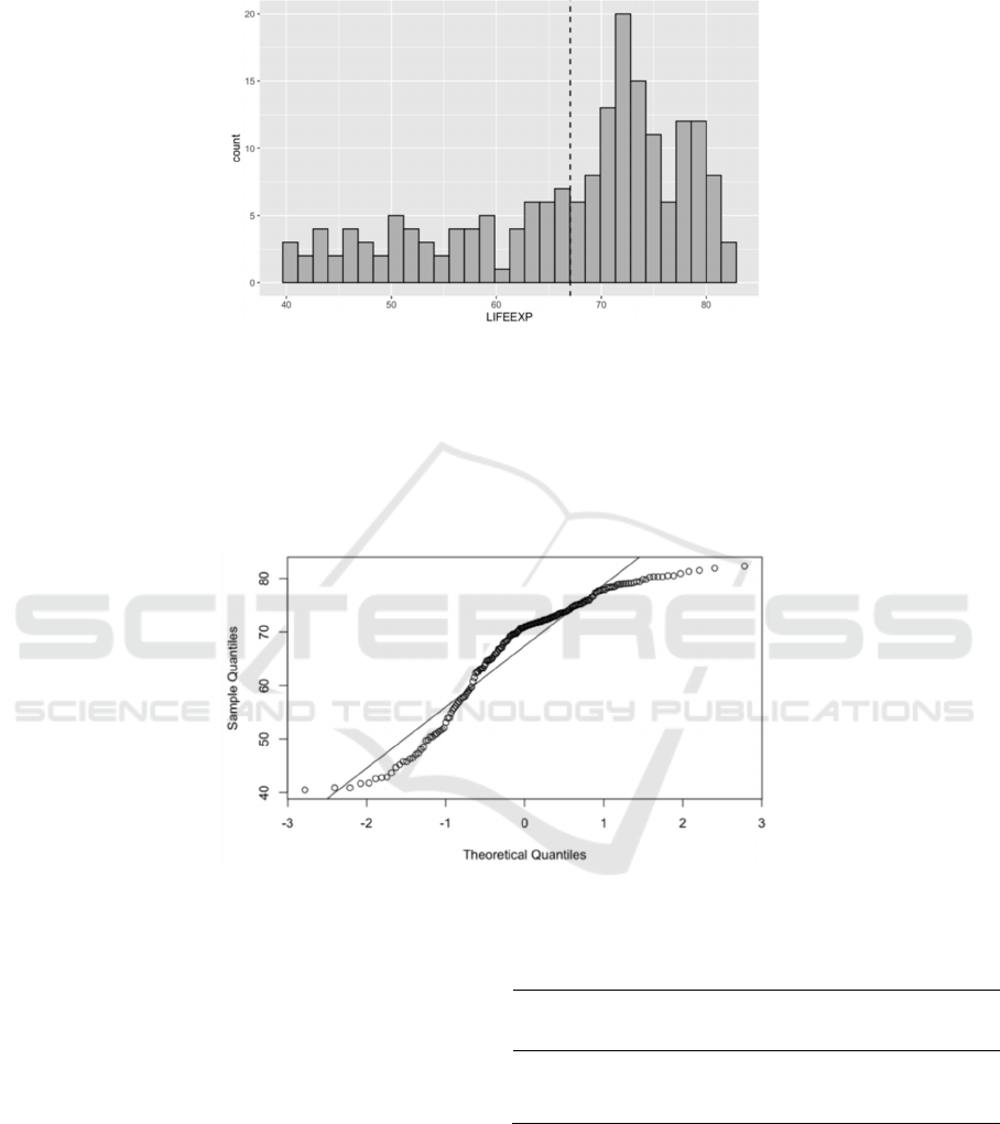
variable has no obvious symmetrical trend and

cannot be considered as normal distribution. Then

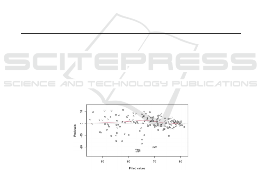
we further use the QQ plot to test in Figure2.

Figure 1: Histogram of LIFRRXP.

When viewing them, the histogram appears to be

skewed to the left. The QQ plot indicates a serious

departure from normality. If we take a natural log

transformation and examine the distribution of this

transformed variable when viewing them, the

transformation still does little to symmetrize the

distribution. It can also be seen from the correlation

matrix that the FERTILITY variable has a strong

correlation with LIFEEXP, and the value in the

correlation coefficient matrix is the largest, so we

can consider establishing a simple linear model of

these two variables.

Figure 2: QQplot of LIFRRXP

3 MODEL ANALYSIS

3.1 A simple Linear Model of Life

Expectancy

We continue the analysis by examining the relation

between y = LIFEEXP and x = FERTILITY. Fit a

linear regression model of LIFEEXP by

FERTILITY. The results are shown as follows.

Table3. Simple linear model regression results

Estimate Std.

Error

t value Pr(>|t|)

(Intercept) 83.7381 1.0439 80.22 <2e-16

FERTILITY -5.2735 0.2887 -18.27 <2e-16

Through observation, we found that p-value <

2.2e-16, so fertility variables have a significant

impact on life expectancy. The obtained linear

model formula is as follows.

LIFEEXP  𝛽



𝛽



 𝐹𝐸𝑅𝑇𝐼𝐿𝐼𝑇𝑌

 5.2735𝐹𝐸𝑅𝑇𝐼𝐿𝐼𝑇𝑌  83.7381

(1)

Linear Analysis of National Life Expectancy

619

3.2 A Multiple Linear Regression

Model of Life Expectancy

After considering establishing a simple univariate

linear model, we will consider using the basic

multivariate linear regression model. According to

the analysis and observation of the missing values of

the data, we found that the variables

RESEARCHERS, SMOKING, and FEMALEBOSS

have many missing values, so these columns of

variable values should be deleted when establishing

the model.

And we can find that the means and standard

deviations of the HEALTHEXPEND variable and

the GDP variable in the data set are large, more than

several hundred times those of the other variables.

At this point, we should consider a log-transformed

form. Taking logarithms of the variables in the

linear regression model can reduce the absolute

differences between the data and the effect of

individual extreme values.

Then we use the filtered variables to establish a

multivariate linear model. However, not every

variable in the model has significant meaning, so we

need to carry out stepwise regression to further

screen and analyze. From the results of stepwise

regression that after two rounds of regression, the

variable FERTILITY, PUBLICEDUCATION, and

lnHEALTH are significant in the model. So next we

consider fitting the regression model with these

three variables. The result is in Table4 as follows.

Table 4: Multiple regression model results.

Estimate Std. Error t value Pr(>|t|)

(

Interce

)

60.7626 4.5865 13.248 < 2e-16

lnHEALTH 3.2777 0.5864 5.589 1.09e-07

PUBLICEDUCATION -0.5341 0.2549 -2.095 0.0379

FERTILITY -3.2220 0.4934 -6.531 1.02e-09

As we expected in Table3, each variable is

signiﬁcant in the model. The expression of the

established multivariate linear model is as follows.

LIFEEXP

β



β



lnHEALTH

β



PUBLICEDUCATION

β



FERTILIT

(2)

 60.7626  3.278lnHEALTH

 0.534PUBLICEDUCATION

 3.222FERTILIT

Also we can do diagnosis plots with this model.

The results are in Figure3, Figure4, Figure5,

Figure6. It shows that most assumptions on the

linear models are consistent with the data

information.

Figure 3: Residuals vs Fitted.

ICEMME 2022 - The International Conference on Economic Management and Model Engineering

620

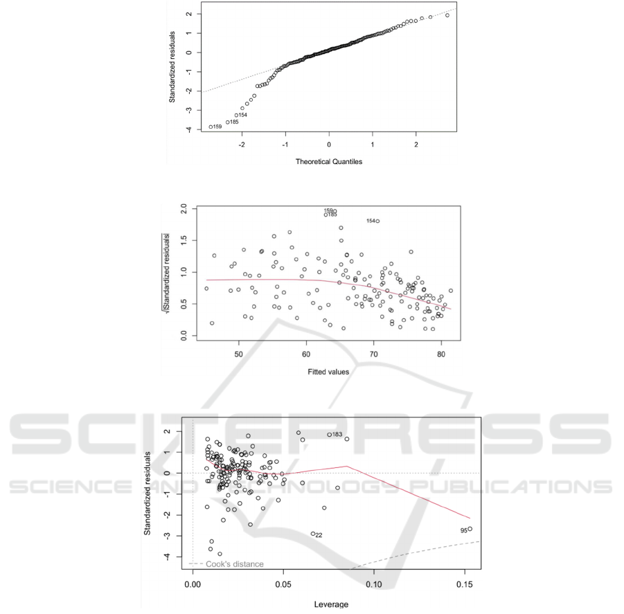
Figure 4: Normal QQplot.

Figure 5: Scale-Location.

Figure 6: Residuals vs Leverage.

Speciﬁcally, we conclude the following:

1.First, the standardized residuals have no

apparent trend in its ﬁtted values. Thus, the

heteroscedasticity of the response variable is not

signiﬁcantly shown.

2. Second, we see that the normality of the

residuals seems acceptable according to the normal

QQ plot, besides the 154th,159th and 185th

observations. Since the empirical quantile based on

normal distribution is fairly close to the theoretical

quantile.

3.Finally, we can see that there is no correlation

between the residual series and prices. Therefore,

the independence assumption seems to be

acceptable.

3.3 Model Improvement and Variable

Selection

The study in the previous section shows that

national life expectancy is significantly associated

with the total fertility rate, public expenditure on

education, and 2004 health expenditure per capita.

As we want to explore how the national life

expectancy changes and differs in regions and

Linear Analysis of National Life Expectancy

621

potential health care systems, in this section we will

add the region variable to the model.

Then we added the categorical variable REGION

to the initial model and again performed stepwise

regression to ﬁlter the new model. From the results,

we found that FERTILITY, REGION,

PHYSICIAN, PUBLICEDUCATION and

lnHEALTH have a signiﬁcant impact.

We take the Variance Inﬂation Factor to check if

there is any obvious collinearity. As we know the

larger VIF implies high correlation between the

independent variable and the remaining variables. It

means that different combinations of the covariates

may lead to the same ﬁtted values, which is

therefore mainly a problem for interpretation rather

than prediction, and cause numerical problems

during the ﬁtting process. For this model, variable

PHYSICIAN has a VIF of 2.60. and a maximum

correlation of 70.1% with the other variables.

Therefore, the removal of this variable could be

considered for the model.

Then we ﬁt a regression model using three

explanatory variables, FERTILITY,

PUBLICEDUCATION, and lnHEALTH, as well as

the categorical variable REGION. The result is in

Table5.

Table 5: Multiple regression model results (add REGION).

Estimate Std. Error t value Pr(>|t|)

(Intercept) 61.4123 64.3493 14.120 < 2e-16

PUBLICEDUCATION -0.5492 0.2416 -2.273 0.0245

lnHEALTH 3.8136 0.5702 6.688 4.58e-10

FERTILITY -3.0003 0.4705 -6.376 2.28e-09

REGION -0.8802 0.2100 -4.191 4.80e-05

All variables are signiﬁcant in this model. And

the expression of the established multivariate linear

model is as follows.

LIFEEXP  β



β



lnHEALTH β



PUBLICEDUCATION β



FERTILITY  β



REGION

 61.4123  3.8136 lnHEALTH  0.5492 PUB  3.000FER  0.880REGION

(3)

Clearly, this model explains the data very well.

The coefficient of determination is 73% and each

variable has a signiﬁcant impact on life expectancy.

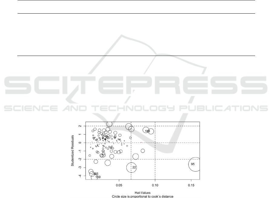
We also can use Cook’s distance to further draw the

inﬂuence diagram to observe some outliers in Figure

Figure 7: Influence Plot.

3.4 Modeling and Screening of

Generalized Linear Models

The generalized linear model is an extension of the

linear model and establishes the relationship

between the mathematical expectation of the

response variable and a linear combination of

predictor variables through a linkage function. It is

characterized by the fact that the natural measure of

the data is not forcibly altered and the data can have

a non-linear and non-constant variance structure. It

is a development of the linear model in the study of

non-normal distributions of response values and the

concise and direct linear transformation of non-

linear models.

ICEMME 2022 - The International Conference on Economic Management and Model Engineering

622

In this problem, we can also consider the

modelling of generalised linear models. We use

different link functions and families to build the

corresponding models and thus compare them to

obtain the best model. Because the join function

involves a logarithmic link function, the

HEALTHEXPEND variable is not treated

logarithmically in this question.

Do the glm LIFEEXP and

PUBLICEDUCATION+HEALTHEXPEND+FERT

ILITY+REGION. The result is in Table6 below.

Table 6: Results of generalized linear model.

EDM

g(μ)

𝛽



𝛽



𝛽



𝛽



AIC

Gaussian Identity -0.451 0.004 -4.246 -1.369 950.2

Gamma Identity -0.608 0.005 -4.043 -1.531 982.9

Inverse Gaussian Identity -0.699 0.005 -3.928 -1.625 1004

Gaussian Log -5.092 e-03 5.255 e-05 -7.115 e-02 -2.012 e-02 954.4

Gamma Log -7.395 e-03 6.002 e-05 -6.988 e-02 -2.269 e-02 985.6

Inverse Gaussian Log -8.779 e-03 6.465 e-05 -6.884 e-02 -2.416 e-02 1006

Then we can ﬁnd the gaussian response with

identity function seems most appropriate, since both

regression parameters are signiﬁcant for modelling

LIFEXP, and the AIC is the smallest among all the

models.

Interestingly, we know that the Gaussian

distribution is approximated as a normal

distribution. That said, if we use the above variables

to build a linear model, a multivariate linear model

might work better than a generalised linear model,

as not every variable is suitable for modelling using

a logarithmic link function. Whether there is a more

appropriate generalised linear model deserves

further research and investigation.

4 CONCLUSION AND

DISCUSSION

In this paper, we ﬁrst conducted a descriptive

analysis of the data, observing the missing value

characteristics of some variables. The correlation

matrix of the data was then derived, and a simple

linear model was developed and analyzed for the

most highly correlated variables. We then built a

multiple regression model using stepwise regression

to explore which potential variables had a more

signiﬁcant effect on life expectancy and test the

model’s feasibility and plausibility. After analyzing

this model, we added the region variable, a

categorical variable with signiﬁcantly different

means across regions. After building a new model

using stepwise regression, we found that region,

fertility rate, healthcare costs, and public education

expenditure signiﬁcantly affected national life

expectancy. Finally, generalized linear models with

different link functions were developed for

comparison and further analysis.

However, this article still has some

shortcomings, such as the treatment of the selection

of variables by deleting columns with many missing

values. It is worth further debating how to

supplement the missing values. As well as in the

generalized linear model, there is no better choice of

linking function, and the form of the link function

still needs further determination. Finally, I believe

that the established multivariate linear model R

can

still be further improved, and in the future, we may

conduct further research.

REFERENCES

Dirac P. (1953) The lorentz transformation and absolute

time. Physica, 19:888–896.

https://doi.org/10.1016/S0031-8914(53)8009 9-6

Feynman R, Vernon F. (1963) The theory of a general

quantum system interacting with a linear dissipative

system. Annals of Physics, 24:118–173.

https://doi.org/10.1006/aphy.2000.6017

Frees E. (1993) Regression modeling with actuarial and

financial applications. Cambridge University Press,

London. https://doi.org/10.1017/CBO9780511814372

Lima M, Siqueira H, Moura A, Hora E, Brito H, Marques

A, et al. (2020) Temporal trend of cancer mortality in

a Brazilian state with a medium Human Development

Index (1980–2018). Sci Rep. 10(1):213-284.

https://doi.org/10.1038/s41598-020-78381-4

Perry K. (2020) Structuralism and Human Development:

A Seamless Marriage? An Assessment of Poverty,

Production and Environmental Challenges in

CARICOM Countries. International Journal of

Political Economy.49(3):222–242.

https://doi.org/10.1080/08911916. 2020.1824735

Linear Analysis of National Life Expectancy

623