3D Semantic Scene Reconstruction from a Single Viewport

Maximilian Denninger

1,2 a

and Rudolph Triebel

1,2 b

German Aerospace Center (DLR), 82234 Wessling, Germany

Technical University of Munich (TUM), 80333 Munich, Germany

Keywords:

3D Reconstruction, 3D Segmentation, Single View, Sim2real.

Abstract:

Reconstructing and understanding our environment is fundamental to human nature. So, we introduce a novel

method for semantic volumetric reconstructions from a single RGB image. Our method combines reconstruct-

ing regions in a 3D scene that are occluded in the 2D image with a semantic segmentation. By relying on a

headless autoencoder, we are able to encode semantic categories and implicit truncated signed distance ﬁeld

(TSDF) values in 3D into a compressed latent representation. A second network then uses these as a recon-

struction target and learns to convert color images into these latent representations, which get decoded during

inference. Additionally, we introduce a novel loss-shaping technique for this implicit representation. In our

experiments on the realistic benchmark Replica-dataset, we achieve a full reconstruction of a scene, which is

visually and quantitatively better than current methods while only using synthetic data during training. On top

of that, we show that our method can reconstruct color images of scenes recorded in the wild. So, our method

allows reverting a 2D image projection of an indoor environment to a complete 3D scene in novel detail.

1 INTRODUCTION

Understanding our surroundings through vision is one

of the fundamental tasks for a visual perception sys-

tem used by any artiﬁcial structure or natural being.

This skill allows a mobile robot to plan and navigate

indoor space. We can achieve this by reverting the

camera’s projection from 3D to 2D. So, we propose

in this work a novel method to reconstruct a 3D scene

from a 2D color image, including the non-visible ar-

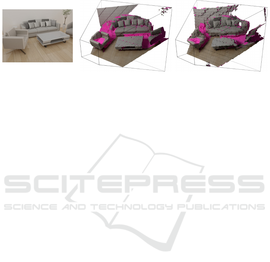
eas. In ﬁg. 1, these non-visible areas from our single

camera view are highlighted in pink. On top of the

full scene reconstruction, we semantically segmented

our reconstructed scene simultaneously. Using only a

single color image, we avoid expensive depth sensors

and reduce the cost of our vision system. Addition-

ally, we remove the requirement of capturing several

images of our scene, as this hinders the quick and easy

use of applications down the line. Our approach can

be applied in many different ﬁelds, from augmented

reality, allowing the overlay of information in the re-

constructed map, to robotics, where it can enable the

planning in unknown scenes.

Our main contributions are:

https://orcid.org/0000-0002-1557-2234

https://orcid.org/0000-0002-7975-036X

• 3D semantic scene reconstruction from one image

• Implicit semantic representation for 3D scenes

• Novel loss shaping for latent reconstructions

2 RELATED WORK

2.1 Scene Compression

Scene compression is a crucial part of this work, as

we store our 3D scenes in a compressed latent for-

mat, which is used as a target for our scene recon-

struction network. Prior works such as DeepSDF

(Yao et al., 2021) and many others (Jiang et al., 2020;

Davies et al., 2020; Chen et al., 2021b) have shown

that implicit TSDF reconstruction is possible. These

reconstructions are converted back into a mesh us-

ing a marching cubes algorithm (Lorensen and Cline,

1987) or a neural network, as presented by Chen et

al. (Chen and Zhang, 2021). In addition, we incor-

porate the advances done by Chabra et al. (Chabra

et al., 2020) and split our scene into several blocks,

compressing them one by one. Yifan et al. (Yifan

et al., 2021) improved SDF reconstructions by adding

a second step to include high-frequency details. Simi-

lar to Denninger et al. (Denninger and Triebel, 2020),

Denninger, M. and Triebel, R.

3D Semantic Scene Reconstruction from a Single Viewport.

DOI: 10.5220/0011747700003497

In Proceedings of the 3rd International Conference on Image Processing and Vision Engineering (IMPROVE 2023), pages 15-26

ISBN: 978-989-758-642-2; ISSN: 2795-4943

 2023 by SCITEPRESS – Science and Technology Publications, Lda. Under CC license (CC BY-NC-ND 4.0)

Ground Truth

Prediction

Input color image

Figure 1: Reconstruction of a 3D scene based on a single color image. On the right is the output of our method.

we align the output scene with our input color im-

age. Building on these ideas, we incorporate cate-

gories into the implicit TSDF reconstruction and add

a new loss to improve the network’s attention around

the objects’ surface. Furthermore, we highlight how

we compress millions of such blocks to use them as a

target for the scene reconstruction network.

2.2 3D Scene Reconstruction

Many recent works have explored the task of recon-

structing an entire 3D scene. Early works focus on

a simpler version of this problem by reconstructing

only the room layout (Ren et al., 2016; Dasgupta

et al., 2016). Other uses multiple viewports or a video

of a scene (Bo

c et al., 2021; Zhang et al., 2021b;

Yariv et al., 2021; Wang et al., 2021; Oechsle et al.,

2021). Instead, this work relies on a single viewport

(Denninger and Triebel, 2020; Shin et al., 2019; Dah-

nert et al., 2021). Denninger et al. (Denninger and

Triebel, 2020) proposed a method to directly map a

2D color image into a 3D scene, where the trans-

formation from 2D to 3D is learned; we build our

approach based on their ﬁndings. Likewise, Shin et

al. (Shin et al., 2019) reconstructed a scene based on

a single color image inside the camera frustum. In

contrast, other methods like Dahnert et al. (Dahnert

et al., 2021) lift the 2D features into the 3D space by

using the camera’s intrinsic parameters and then re-

constructing the scene. Zhang et al. (Zhang et al.,

2021a) proposed a similar method, where one CNN

detects the objects and a second one their pose. A

third CNN then uses this information to optimize their

shape in 3D. The Mesh-RCNN (Gkioxari et al., 2019)

by Gkioxari et al. relies on estimating the pose of

the objects in a scene, and then they reconstruct their

shape. However, this does not include the reconstruc-

tion of the entire scene. Kuo et al. (Kuo et al., 2020)

instead rely on a CAD model retrieval approach rather

than a generative approach for the objects. We instead

propose to learn the 2D to 3D transformation and pre-

dict the entire scene at once, avoiding the problem of

setting a threshold for the bounding box detector. In-

stead of a color image Song et al. (Song et al., 2016)

used a depth image to perform a 3D semantic scene

reconstruction. Our approach also produces a 3D se-

mantic segmentation without relying on the propaga-

tion of 2D features. In contrast to NeRF from Milden-

hall et al. (Mildenhall et al., 2020), and its many

derivatives (Martin-Brualla et al., 2020; Chen et al.,

2021a; Barron et al., 2021; Mildenhall et al., 2021;

Xu et al., 2022), we only use one single color image

of a scene without knowing the camera’s pose.

3 SCENE REPRESENTATION

3.1 Problem Deﬁnition

We deﬁne our problem as a mapping from 2D image

coordinates p

= (x

) to 3D scene coordinates p

). Here, each ﬁnal 3D coordinate has a trun-

cated signed distance ﬁeld value (TSDF) and the cat-

egory of the closest surface. The input is an RGB im-

age I

: Ω

→



[0,255]



; Ω

⊂ R

and a generated

surface normal image I

: Ω

→



[−1,1]



, where Ω

is the set of image coordinates. This means that we

can evaluate our network Θ for a given 3D scene co-

ordinate p

and an image I =

{

)| p

∈ Ω

}

with:

Θ :

{

(Ω

)

}

× R

→ R × N (1)

(I , p

) 7→ Θ(I , p

) = (t,c) | t ∈ [−σ, ··· , σ] , c ∈ N

(2)

Here the result for each point p

is the TSDF value

t and the category label c. This TSDF value is the

signed distance to the closest surface and can not be

smaller than the truncation threshold −σ or bigger

than σ. It is also positive outside of objects and neg-

ative inside of them. In contrast to a ﬁxed voxel grid,

IMPROVE 2023 - 3rd International Conference on Image Processing and Vision Engineering

we can evaluate the scene at an arbitrary resolution

and are only bound by the network’s capacity.

Our TSDF values are stored view independent,

corresponding to a complete TSDF approach, where

the distance is zero on the surface and σ in the free

space. This so-called complete view contrasts a pro-

jected TSDF approach, where the distance is only cal-

culated along the camera view axis, e.g. Dahnert et

al. (Dahnert et al., 2021). However, such a projected

view contains considerable jumps in the TSDF space,

while a complete TSDF space is smooth, even though

it is more challenging to compute.

Inspired by Denninger et al. (Denninger and

Triebel, 2020), we also use a perspective transfor-

mation to map a 3D scene into a cube C = [−1,1]

This mapping is done using the camera’s pose matrix

extrinsic

followed by the perspective camera matrix

intrinsic

built from the known camera intrinsics. We

set the near-clipping plane to one meter and the far

one to four meters. After mapping our scene into the

cube, each color pixel corresponds to an axis-aligned

line in the cube. However, this perspective trans-

formation also introduces a distortion along the Z-

axis, making objects closer to the camera larger in Z-

direction than objects farther away, see a) - c) in ﬁg. 2.

We remove this distortion by applying the square root

to the Z-coordinate z

of the points p

, leading to d) in

ﬁg. 2. As z

∈ [−1; 1], we ﬁrst need to scale it to the

range [0;1] and afterwards to [−1;1]:

←

+ 1)/2 · 2 − 1 =

+ 2 − 1 (3)

This transformation improves the distribution in

Z-direction for our speciﬁc depth range while trans-

forming ﬂat surfaces to curved ones, see d) in ﬁg. 2.

3.2 Semantic TSDF Point Cloud

Generation

We create our own dataset, as none exists, which maps

2D images to sematic TSDF point clouds. Such a

point cloud should have TSDF values and semantic

labels around the surface of each object. For this,

we extend the SDFGen tool (Denninger and Triebel,

2020), as the original version only works on TSDF

voxel grids. At ﬁrst, we add a semantic label to all

polygons and then rely on the octree combined with

a ﬂood ﬁll of the SDFGen tool to compute a TSDF

voxel grid with a shape of 128

. This voxel grid

is used to detect the free and occluded areas in our

scene, a) in ﬁg. 2. To later check whether a point is

inside an object, we sample anchor points in the free

space, b) in ﬁg. 2. To create our TSDF point cloud

around the objects, we start by sampling points on

the surface areas reachable from the camera. This

sampling is necessary as some polygons or part of

them are occluded, e.g. a couch hidden behind a wall.

We only want to reconstruct reachable objects of the

scene, nothing that lies behind a wall in a different

room. So, we deﬁne that a point p

on a polygon is

visible if at least three anchor points are reachable

from p

without intersecting any polygon. We use

three points to avoid extending the reachable space

through thin gaps. For example, the inside of a cup-

board with an open slit could be otherwise accessed.

As we aim to reconstruct scenes, we assume that the

objects’ insides are ﬁlled. These points then deﬁne

our surface, see c) in ﬁg. 2. To correct the distortion

from the K

intrinsic

, we use eq. (3) and get d) in ﬁg. 2.

We can now generate our desired TSDF points by

randomly taking a surface point and adding a random

direction vector with the length of 2σ, see g) in ﬁg. 2.

We then determine the TSDF value for each newly

created point by ﬁnding its closest surface point with a

nearest neighbor search. However, the resulting point

is most likely not the closest point on the surface of

the curved polygon, as we only have a ﬁxed amount

of surface points. We can ﬁnd a closer surface point

by sampling around our original surface point on the

curved polygon. This process gets repeated until the

distance converges. We take the category from the

corresponding curved polygon. In the end, the sign of

the TSDF value is based on the visibility to an anchor

point. We repeat this for a ﬁnal amount of 2,000,000

points per scene, calculating the TSDF value and cat-

egory per point, see f) in ﬁg. 2.

To enable the alignment of our scene with the im-

age, we voxelize our created points. Using a res-

olution of 16, we get a good compromise between

the number of blocks and the structural details in-

side a block, see g) in ﬁg. 2. We increase the block

size by a boundary factor b of 1.1 in every direc-

tion to make it easier to compress these blocks in

the next step. Points on the boundary are there-

fore included in more than one block. The code

for all can be found here: https://github.com/DLR-

RM/SemanticSingleViewReconstruction.

4 SCENE COMPRESSION

These voxelized blocks of point clouds need to be

brought into a latent representation to train our scene

reconstruction network. We follow a similar route as

DeepSDF and Deep local shapes (Yao et al., 2021;

Chabra et al., 2020) by compressing each block ﬁlled

with TSDF points into one latent vector using an im-

plicit TSDF representation. Our addition here is the

3D Semantic Scene Reconstruction from a Single Viewport

reconstruction of the category for each given point

and our unique loss-shaping technique.

At ﬁrst, we learn a transformation of our 3D point

into 128 values on which a Fourier transformation is

used, inspired by Tancik et al. (Tancik et al., 2020).

We concatenate this with the 512 values long latent

vector l for this block. This combined input vector

is forwarded through two layers of size 512 and 128,

each using a RELU activation. For the TSDF output

t, we only use a ﬁnal layer to reduce the size down

to one value, whereas, for the class output, we rely

on two fully connected layers with a length of 16 and

then down to the number of classes

. This architec-

ture is depicted in ﬁg. 3.

Our novel loss function here incorporates the pre-

diction of the TSDF value and the category class,

which can be seen in eqs. (4) and (5). We start by tak-

ing the absolute difference between the TSDF label

tsdf

and the TSDF output t of the network, resulting

in L

dist

. Using a standard category loss, we combine

the network’s category outputs c and the desired one

hot encoded category labels y

. The combination of

these losses is discussed in section 6.

dist

tsdf

−t

(4)

= −

∑

i=1

[i] · log (c[i]) (5)

For the training, we initialize the latent vector l

with zeros to ensure that the output is deterministic for

a given point cloud. We then optimize only the latent

vector for 2048 points per block for 1400 steps. Af-

terward, the network weights get optimized with the

frozen latent vector l for another 1400 steps. This pro-

cess is repeated for new blocks until the network con-

verges. All hyperparameters used here are found by

optimizing 7.259 networks, as the performance and

computation time are crucial.

As we compress an entire scene with a side res-

olution of 16, our compressed space has a size of

× 512 latent values, as each block gets com-

pressed into 512 values. So for each scene, we need

to perform 1400 latent update steps to optimize the

latent vector for our 16

= 4096 blocks, whereas each

a) Meshed voxelgrid 128 b) Anchor points c) Surface points

d) Surface points

Z corrected

e) Sampled points f) TSDF sampled points g) Blocked TSDF sampled points

Figure 2: Creating a blocked TSDF point cloud around the reachable surface. First, SDFGen (Denninger and Triebel, 2020)

creates a low-resolution voxel grid (a). In its free space, anchor points are sampled (b). These anchor points determine whether

a sampled surface point is reachable (c). We then remove the Z-compression (d) and sample new points around our surface

points (e). Finally, we determine the distance to the curved surface (f) and divide it into different blocks.

IMPROVE 2023 - 3rd International Conference on Image Processing and Vision Engineering

512

128

512

128

t: TSDF output

c: class output

Input

Legend:

Fourier transformation

Fully connected layers

TSDF and class output

Figure 3: Compressing the implicit semantic representation.

block contains 2048 points. On an Nvidia RTX 3090,

1400 steps take 1.15s per block. For 89,029 scenes

with 4096 blocks, this would take 13.3 years. To

speed this up, we split our scene into three parts:

boundary, non-boundary, and free/ﬁlled. For this, we

save a voxel grid during the TSDF point cloud gen-

eration, with a resolution of 256 of the Z-corrected

scene. This grid is created by calculating the TSDF

and semantic value for the voxel grid points. As most

are in free space, they can be ﬁlled by checking the

visibility to an anchor point.

We spend the most time on the boundary blocks,

ensuring that the TSDF values precisely follow the

object’s surface and assign the correct category. The

non-boundary blocks are much easier as they usually

only have a simple gradient in one direction, making

it easier to optimize the corresponding latent vector

l. For the ﬁlled and empty blocks, which don’t con-

tain any points, we can assign the corresponding la-

tent vector, which is predicted only once. All the ﬁlled

and empty regions get the category ”void” as they are

too far from a surface to predict a category. We start

with an estimated latent vector to speed up the predic-

tion for the boundary and non-boundary blocks. This

latent vector is part of a database of 1,483,472 blocks

(750 scenes) with the total 1400 steps we calculated

prior. So during the calculation of the rest, we ﬁnd

the most similar block in the database for each new

block and use its latent vector as an initialization. The

similarity is compared by voxelizing the block’s point

cloud with a resolution of four into 64 blocks and then

averaging the TSDF values of these voxels. We then

add ten more elements containing our category distri-

bution for the block and compare this 74-long vector

via a KDTree to the vectors in the database.

These pre-initialized latent vectors then reduce the

number of optimization steps for boundary blocks

from 1400 to 750. Further, we stop early if the ab-

solute error on the TSDF values is below 0.02, which

we check every 125 steps. For the non-boundary

blocks, the database reduced the number of steps to

160, where we check every 20 steps if the absolute

TSDF error is below 0.03 and move on to the next

block if that is the case. With this reduction, we only

have to predict half of the blocks, while each block

only takes an average of 0.3s. So, the time on a sin-

gle GPU is reduced to only 1.27 years or roughly nine

days on 50 GPUs, giving us a compressed latent rep-

resentation that can be used in the next step.

5 SCENE RECONSTRUCTION

The ﬁnal goal of this work is the reconstruction of an

entire 3D scene based on a single color image. As

our reconstruction target, we use the 16

× 512 latent

blocks generated in section 4. We rely on the tree-

net architecture by Denninger et al. (Denninger and

Triebel, 2020) but adapt it to a smaller spatial output

resolution of 16 in contrast to 32.

An overview of our network is given in ﬁg. 4. The

input to our network is a color image and a surface

normal image as the normal image guides the recon-

struction of ﬂat surfaces. During inference, this sur-

face normal image is generated by a simple U-Net

based on the color image, while during training, we

rely on the synthetic ground truth. After concatenat-

ing both inputs, it is forwarded through ﬁve convolu-

tions and max poolings to reduce the spatial resolu-

tion from 512 down to 16 and increase the number of

feature channels from 6 to 512. We can transform a

2D image into a 3D tensor using the tree-net archi-

tecture. Each path from the tree root to a leaf cor-

responds to a 3D depth slice of the camera frustum,

while each node uses two ResNet blocks, with two

convolutions each (He et al., 2016). This design en-

ables the network to learn speciﬁc feature sizes and

propagate this information to the correct slice posi-

tion. We then combine all leaves in 3D, where each

leaf is only responsible for a particular 3D slice in Z-

direction. The channels of such a leaf are distributed

over several 3D tensors, creating an output 3D voxel

with a size of 16

× 512. On this combined 3D out-

put, we perform eight 3D convolutions with 512 ﬁl-

ters each to enable smoothing and cross-talk between

the single paths of the tree, avoiding that a failure

of one path decreases the performance of the whole.

We rely on inception layers to increase the receptive

ﬁeld; however, we increase the dilation rate instead of

the ﬁlter size (Yu and Koltun, 2015; Denninger and

Triebel, 2020). So, we split the number of feature

channels for each convolution and use half with a di-

lation rate of 1 and the other half with 2.

3D Semantic Scene Reconstruction from a Single Viewport

Input

U-Net

512

256

128

256

512

reconstructed scene

for each 1

512 vector use

the decoder and

then unproject it

Conv2D + Pooling

2 × ResNet block

Combined 3D result

Conv3D

Figure 4: Our proposed architecture uses one image and reconstructs an entire 3D scene.

6 LOSS SHAPING

A crucial step to focus the attention of the network

on the relevant reconstruction targets is loss shaping

(Denninger and Triebel, 2020). Here, we increase the

loss in parts of the scene where the network should

perform well. This increase is necessary as the solu-

tion space we try to regress is enormous.

6.1 Scene Compression

We introduce three losses to improve the reconstruc-

tion accuracy for the scene compression. The ﬁrst

one sharps the loss around the surface. The second

one increases the loss in relation to the distance to

the blocks’ boundaries, which reduces block artifacts.

And the last one ensures that the gradient is constant

over the reconstruction space.

Denninger et al. (Denninger and Triebel, 2020)

rely on a Gaussian distribution to strengthen the loss

around the surface. Instead, we design an inverse

function, which uses our surface loss weight θ

surface

and the truncation threshold σ, deﬁned by the gener-

ation process in section 3. Here, y

tsdf

is the desired

output for a given point p, and t is the output gener-

ated by the network deﬁned in section 4. Increasing

the loss if the current point p is close to a surface,

meaning that its y

tsdf

is close to zero. The results are

best if θ

surface

is set to 37.27 and ε to 0.001.

surface

= L

dist

surface

· σ

tsdf

+ ε

(6)

Additionally, we increase the loss in relation to the

distance to the blocks’ boundaries. By determining

the closest distance along the axis of one point p to

the sides of the projection cube C . We do this by tak-

ing the minimum and maximum value of the point p

and comparing it to the boundary b. The closest dis-

tance d

cube

is used, and 1.0 is subtracted from it to

increase the loss as it approaches the boundary. The

ﬁnal result L

boundary

is squared to sharpen the edges.

These are deﬁned in eq. (7) and eq. (8), and visualized

in ﬁg. 5. Here, the boundary factor b depends on the

block scaling deﬁned in section 3.2.

min dist

= min



b + min

i∈[1,2,3]

p[i], b − max

i∈[1,2,3]

p[i]



(7)

boundary

= L

dist

· (1.0 − d

min dist

)

(8)

inverse distance

Combining all of them then results in our com-

bined loss L

combined

, which can be seen in eq. (9).

Here, the category weight θ

combines the two dif-

ferent loss heads. Our extensive search with 7.259

tests found that a value of 30.31 for θ

works best.

combined

= L

dist

+ L

surface

+ L

boundary

+ θ

· L

(9)

Our last addition to the loss ensures that the

sparse TSDF input points provided to the network

are smoothly interpolated. We propose to punish

high-frequency signals between two neighboring in-

min dist

inv. distance

boundary

-1.1 -0.7 -0.3 0.0

point value p[i]

0.3 0.6 1.0

0.00

0.25

0.50

0.75

1.10

Figure 5: The different results for the three parts deﬁned in

eq. (7) and eq. (8) are shown here.

IMPROVE 2023 - 3rd International Conference on Image Processing and Vision Engineering

Table 1: Results of our TSDF compression method.

Method Prec Rec IOU CD

Class

Acc.

Without L

surface

95.76 95.49 91.74 0.0034 99.57

With L

Gaussian

97.08 97.53 94.81 0.0030 99.65

Without L

boundary

98.98 98.94 97.92 0.0015 99.65

Without L

gradient

98.93 98.95 97.91 0.0013 97.73

With

= 256 98.83 98.76 97.63 0.0020 98.94

No categories 98.82 98.75 97.68 0.0013 X

Our method 99.00 98.96 97.93 0.0013 99.67

put points. For this, we add a loss if the gradient of the

point inputs in relation to the combined loss is bigger

than the euclidean distance between two points. This

loss can be seen in eq. (10), where (δL

combined

)/(δp)

is the gradient of the combined loss in relation to the

input point p, and g is the maximum value the gra-

dient can take, in our scenario g is one. We ﬁnally

scale this output with θ

gradient

to ensure that the gradi-

ent stays below the g, achieved by setting θ

gradient

1000.0.

gradient

= θ

gradient

· ReLU



δL

combined

δp

− g



(10)

Our training loss L

tsdf ﬁnal

is the sum of the

combined

and L

gradient

. To show the effectiveness of

our losses, we evaluate them on voxel-based metrics

such as precision, recall, and IOU and also surface

metrics like the chamfer distance and the class accu-

racy in table 1. Removing our proposed L

surface

drasti-

cally hurts the performance on the IOU and the cham-

fer distance from the predicted mesh to the ground

truth, as it focuses the attention on the surface of the

objects. Our L

surface

performs better than the Gaus-

sian loss introduced by Denninger et al. (Denninger

and Triebel, 2020), redeﬁned in eq. (11). In this test,

it only replaces the L

surface

Gaussian

= L

dist

· (N (0,0.25 · σ)(y

tsdf

) · 0.25 · σ)

(11)

The gains for L

boundary

and L

gradient

are smaller

but apparent in a visual inspection, e.g. artifacts are

visible on the boundaries without the L

boundary

. The

gradient

, on the other hand, takes care of ﬂying surface

imperfections in free or occluded space, which re-

sult from high-frequency changes in the TSDF space.

When the latent vector size is reduced from 512 to

256, the classiﬁcation error shows a large increase.

As we use these latent vectors as the regression tar-

gets for our scene reconstruction network, they form

the upper boundary of our ﬁnal 3D scene reconstruc-

tion performance.

6.2 Scene Reconstruction

First, we make the process more dynamic than prior

solutions for scene reconstruction (Denninger and

Triebel, 2020) by precalculating a loss grid at a res-

olution of 256, which is dynamically mapped to the

loss values during training. This dynamic mapping

allows us to change the used loss values after gen-

eration. We also integrated the class value into the

precalculated loss value, allowing us to increase the

loss around objects in contrast to the ﬂoor, ceiling,

and walls in a scene.

We rely on the projected TSDF voxel grid gener-

ated in section 3, where we extract the classes for the

2,000,000 points and store them in a 3D grid with the

same 256 resolution as the TSDF voxel grid. The cat-

egory for each voxel is based on the majority of points

in this voxel. For detecting the free visible space, we

walk along the camera rays into the 3D voxel grid and

set all voxels to free until we hit an occupied one, as

can be seen by the white circles in ﬁg. 6. This ﬁrst

occupied voxel is set to true surface. From the free

voxel, we start a ﬂood ﬁll algorithm into the still unde-

ﬁned and free areas. Based on the distance to the clos-

est free voxel k, we assign a free non-visible k value,

depicted by the gray circles in ﬁg. 6. Here, k can be

between 0 and 150 values, roughly 59% percent of the

scene axis. Every occupied voxel we reach with the

ﬂood ﬁll algorithm is set to true non-visible surface.

To focus the attention more on the surface boundary,

we set the 32 values before and 16 after a true surface

to surface. We repeat this for the non-visible surface

values; see the non-ﬁlled stars and pentagons in ﬁg. 6.

Instead of just increasing the loss along the view-

ing direction, we increase it in all directions, boosting

the loss around thin objects. We achieve this by iter-

ating over all true surface values and setting for each

of them in a radius of 16 all free values to surface val-

ues. This is repeated for the non-visible surface val-

ues as well. This change increases the loss, even if the

surface normal is nearly perpendicular to the viewing

direction. Lastly, we combine all surface values with

a category class. Additionally, we increase the loss

for non-ﬂoor or wall values by ﬁve, as objects have a

greater appearance variety than walls and ﬂoors. Fig-

ure 6 shows how the loss shapes around objects and

categories, and the legend contains the values we used

during training. By averaging from 256

down to 16

we can multiply our weight W

surface

with the absolute

difference between the network’s output o and the tar-

get labels y, resulting in our reconstruction loss:

rec

= W

surface

512

∑

i=0

− y

(12)

3D Semantic Scene Reconstruction from a Single Viewport

To ensure that the 3D structure is learned before

the 3D convolutions are applied, we introduce a tree

loss L

tree

. This loss takes the input to the ﬁrst 3D layer

and passes it through a 3D convolution with a ﬁlter

size of 512 matching our y. This output o

tree

is then

compared to y the same way as for o in eq. (12) and

then multiplied with our W

surface

. The resulting L

tree

is scaled with a factor of 0.4 before combining it with

rec

to form our training loss L: L = L

rec

+ L

tree

· 0.4

7 DATASET & EXPERIMENTS

7.1 Replica and 3D-FRONT-dataset

Our approach is evaluated on the Replica-dataset

(Straub et al., 2019), while we only trained it on

data from the synthetic 3D-FRONT-dataset (Fu et al.,

2020b; Fu et al., 2020a). For our training, we cre-

ated 84,508 color- and predicted surface normal im-

ages and corresponding compressed voxel grids with

a matching loss weight θ

surface

. The camera poses in

the 3D-FRONT scenes, and the color and ground truth

surface normal images are generated using Blender-

Proc (Denninger et al., 2019). We focus on ensur-

ing that each camera’s view contains various objects

and that the overlap between two camera poses in the

same scene is small or non-existent by calculating the

distance between projected depth images of the re-

spective camera poses. We limit this maximal dis-

tance between two points in our two points clouds to

0.5m. After 50,000 tries, we reduce it to 0.25m. Fur-

ther, we had to remove 4,619 objects from the 16,563

objects in the 3D-FUTURE dataset, as they were ei-

ther not water-tight or the object normals point in dif-

ferent directions breaking the TSDF generation. We

design a simple U-Net architecture to generate the

predicted surface normal images by training it on the

3D-FRONT-dataset. For details on the U-Net archi-

tecture, see the code.

7.2 Category Reduction

As the overarching goal of this work is to reconstruct

scenes to enable navigation and planning for mobile

robots, we reduce the number of categories to ten be-

cause the difference between various cabinet types in

the 3D-FRONT-dataset is not vital to us. This re-

duction leads us to the following classes: void, table,

wall, bath, sofa, cabinet, bed, chair, ﬂoor, lighting.

7.3 Evaluation

We compare our method to Total3Dunderstanding by

Nie et al. (Nie et al., 2020), Panoptic 3D Scene Re-

construction (P3DSR) by Dahnert et al. (Dahnert

et al., 2021), and to SingleViewReconstruction (SVR)

by Denninger et al. (Denninger and Triebel, 2020).

Using the same camera intrinsics as them, we gen-

erated 20 images per Replica scene, resulting in 360

images. The Replica-dataset was selected as none of

the methods was trained on it, and it contains real-

world recorded scenes. We then compare the unpro-

jected meshes in meters using the chamfer distance

between the ground truth and the predicted

mesh, where we ﬁnd for each point in the ground truth

the closest matching point in the prediction and av-

erage the distances between these matching points.

To calculate the chamfer distance to the prediction

pred

, we switch the two meshes. Our results in ta-

ble 2 show that we achieve a CD

of 10.53 cm and

an IOU of 69.45% on the Replica-dataset. We focus

here on the CD

, as we are more interested in recon-

structing every object than by accident predicting too

much-occluded space, as missing an object might lead

to a collision during navigation. Important to note

here is that we only compare the reconstruction in a

range between 1 and 4 meters as deﬁned in section 3.

However, P3DSR can predict further back than this,

but these results are not considered here. For SVR,

we also compare the voxel-based metrics for the oc-

cupied regions by applying the same Z-correction on

Camera

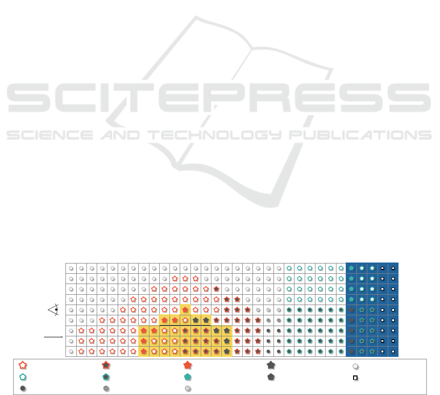
Z-axis

sofa s. : 250 sofa s.n.v. : 50 true sofa s. : 2500 true sofa s.n.v. : 500 free: 2

wall s. : 50 wall s.n.v. : 10 true wall s. : 500 true wall s.n.v. : 100 not reachable: 0.1

lower free n.v. : 0.5 half free n.v. : 0.75 upper free n.v. : 1.0 s.=surface n.v.=non-visible

Figure 6: A top-down 2D view, showing the sofa in yellow, and the wall in blue. The symbols determine the loss values.

IMPROVE 2023 - 3rd International Conference on Image Processing and Vision Engineering

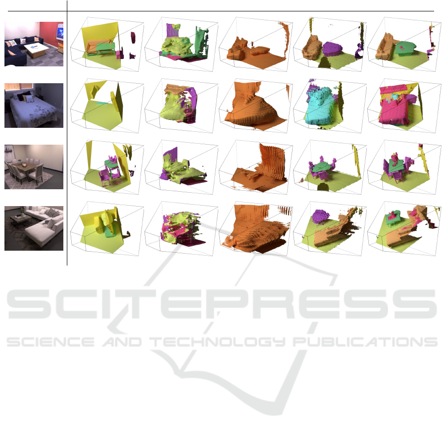
Input

Our methodTotal3D P3DSR SVR GT

cam tilt 69.9

◦

cam tilt 62.4

◦

cam tilt 64.9

◦

cam tilt 58.1

◦

With GT

bounding boxes

no segmentation

Figure 7: Results on the Replica-dataset for four different color images. All methods only use a color image as an input. Our

method Our method shows the best reconstruction, followed by our other presented method SVR.

the voxel grid, as done on the points in eq. (3). This

ensures that the IOU in the cube better reﬂects the

actual scene reconstruction. Another metric is class

accuracy which is the amount of correctly classiﬁed

points, where we map every vertex of our true mesh

to the closest point in the prediction and check if they

share the same category. SVR is not evaluated on that,

as it does not provide a semantic segmentation. We

use the code and pre-trained weights by the authors

for all methods. All methods use only one color image

of the scene, except Total3Dunderstanding, which we

provide with the GT bounding boxes, to avoid affect-

ing the networks’ performance by our chosen bound-

ing box detector. A qualitative evaluation is shown in

ﬁg. 7, where our method outperforms all other meth-

ods in the level of detail and overall reconstruction

performance. However, our method fails to correctly

classify the couch table as a table in the ﬁrst and last

row and predicts a cabinet instead.

SVR and P3DSR are only trained with a ﬁxed

camera tilt of 78.69

◦

and 90

◦

and a ﬁxed camera

height of 1.55m and 90cm, respectively. However,

we evaluate with our validation images, which have a

camera tilt range of 45

◦

to 85

◦

and a camera height

of 1.45 to 1.85m, and show these results in table 2.

Furthermore, to not evaluate the training angle/height,

we regenerate our images at the same position in

the scene but now with a method-speciﬁc angle and

height. Our measured performance drops drastically

at 90

◦

, as we only trained up to 85

◦

. Additionally, at a

low height of 90 cm, most surfaces are perpendicular

to the viewing direction making it particularly hard

to predict their depth. Interestingly the performance

of P3DSR drops as well; we assume this is because

reconstructing at this angle is more challenging.

7.4 Results in the Wild

To show the performance of our method, we collected

images via different phone cameras in ﬁve homes and

show the results in ﬁg. 8. The most remarkable result

is on the left in the second row, containing a dining

table surrounded by chairs. Even though the backside

of the right chair is missing, the network understood

that there must be a chair as the sitting area was recon-

structed, which is not visible in the single color im-

age. Generating a surface normal image, an encoded

3D scene, and decoding this 3D scene with a resolu-

tion of 256 on an Nvidia 3090 RTX takes

≈

0.9s, for

a resolution of 512, it takes

≈

4.2s.

3D Semantic Scene Reconstruction from a Single Viewport

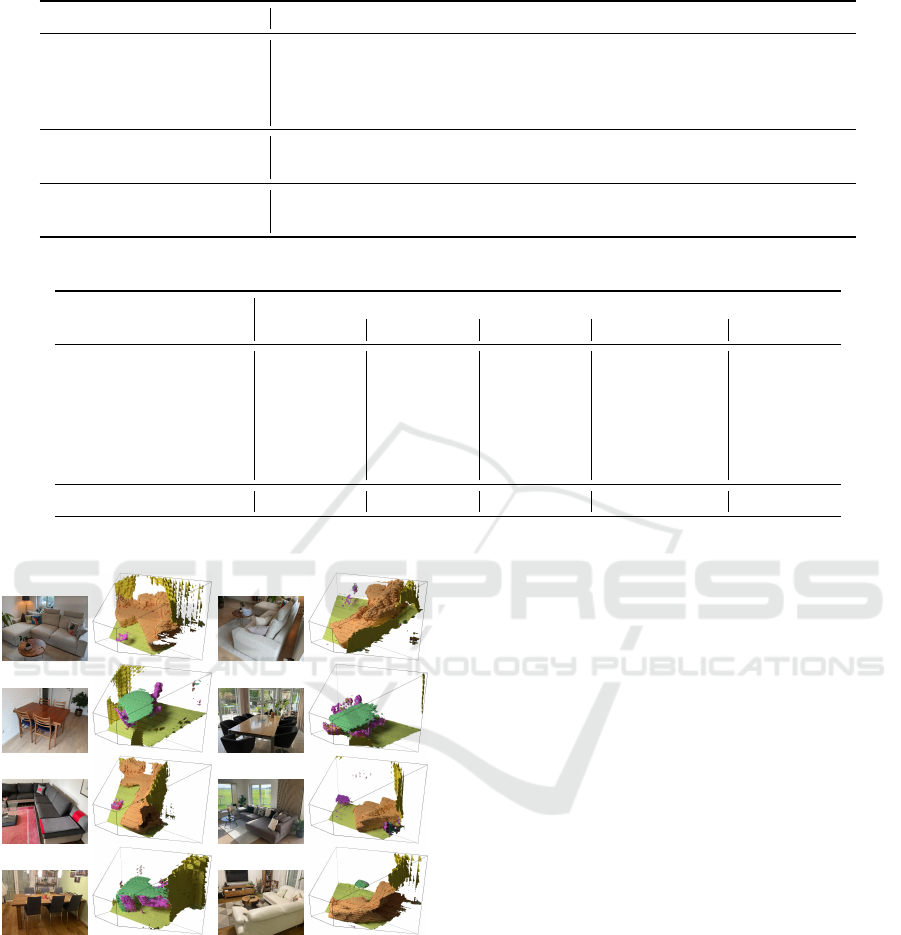
Table 2: Different methods evaluated on the real-world Replica-dataset.

Angle Method Precision Recall IOU CD

pred

Class Acc.

[45

◦

9 80

◦

] Total3D - - - 0.3057 0.3545 32.77

[45

◦

9 80

◦

] P3DSR - - - 0.1728 0.3144 17.49

[45

◦

9 80

◦

] SVR 75.62 60.85 48.28 0.4189 0.4319 X

[45

◦

9 80

◦

] Our method 85.30 79.41 69.45 0.1053 0.2331 66.78

78.69

◦

SVR 86.79 67.30 60.01 0.5168 0.3926 X

78.69

◦

Our method 82.84 76.65 65.46 0.1081 0.2526 64.86

◦

P3DSR - - - 0.1858 0.2692 10.74

◦

Our method 79.97 48.41 41.67 0.3051 0.3751 48.19

Table 3: Ablation study on the Replica-dataset with the GT and generated normals.

Ablation

Precision Recall IOU CD

Class Acc.

GT gen GT gen GT gen GT gen GT gen

Reduced no. 3D ﬁlters 83.0 85.9 86.8 78.3 73.3 69.0 0.088 0.107 64.9 67.1

Without inception 84.2 85.1 84.4 77.0 72.6 67.2 0.085 0.110 62.9 63.6

Without wall weight 83.1 84.1 83.9 76.7 71.3 66.4 0.092 0.111 70.8 68.9

Tree height of two 84.5 85.5 83.5 76.7 72.1 67.5 0.086 0.112 67.5 67.0

Tree height of four 84.2 85.0 82.8 75.3 71.2 65.9 0.088 0.111 67.0 65.8

Without loss shaping 87.1 87.2 85.7 78.0 75.5 69.4 0.148 0.168 77.5 75.5

Our method 84.2 85.3 85.5 79.4 73.3 69.5 0.084 0.105 68.0 66.8

Figure 8: Our method in the wild. Eight images recorded in

ﬁve different homes and their 3D segmented reconstruction.

7.4.1 Ablation

We also performed various ablation studies to show

the effects of our design decisions in table 3. These

results show that our proposed network has the high-

est IOU and lowest CD

value when using generated

normals. Reducing the number of 3D ﬁlters from 512

to 256 barely reduces the CD

performance, indicat-

ing that a quicker method could be designed.

8 CONCLUSION

We presented a novel method to reconstruct and seg-

ment 3D scenes with only a single color image. For

this, we use a neural network to embed part of the

scene with an implicit TSDF representation, which

incorporates the distance and category of the closest

surface. These generated embedded latent vectors for

each part are then used as a target for our scene recon-

struction network. Together with our novel loss shap-

ing techniques, we outperform three current methods

on the challenging and realistic Replica-dataset by

nearly cutting the average measured chamfer distance

in half. Indicating that semantic segmentation and

scene reconstruction with only a single image is pos-

sible in challenging real-world environments while

training only on synthetic data.

REFERENCES

Barron, J. T., Mildenhall, B., Tancik, M., Hedman, P.,

Martin-Brualla, R., and Srinivasan, P. P. (2021). Mip-

nerf: A multiscale representation for anti-aliasing

neural radiance ﬁelds. International Conference on

Computer Vision. 2

c, A., Palafox, P., Thies, J., Dai, A., and Nießner, M.

(2021). Transformerfusion: Monocular rgb scene re-

IMPROVE 2023 - 3rd International Conference on Image Processing and Vision Engineering

construction using transformers. Neural Information

Processing Systems. 2

Chabra, R., Lenssen, J. E., Ilg, E., Schmidt, T., Straub, J.,

Lovegrove, S., and Newcombe, R. (2020). Deep local

shapes: Learning local sdf priors for detailed 3d re-

construction. European Conference on Computer Vi-

sion. 1, 3

Chen, X., Zhang, Q., Li, X., Chen, Y., Feng, Y., Wang, X.,

and Wang, J. (2021a). Hallucinated neural radiance

ﬁelds in the wild. Conference on Computer Vision and

Pattern Recognition. 2

Chen, Z. and Zhang, H. (2021). Neural marching cubes.

ACM Transactions on Graphics. 1

Chen, Z., Zhang, Y., Genova, K., Fanello, S. R., Bouaziz,

S., H

ane, C., Du, R., Keskin, C., Funkhouser, T. A.,

and Tang, D. (2021b). Multiresolution deep implicit

functions for 3d shape representation. International

Conference on Computer Vision. 1

Dahnert, M., Hou, J., Nießner, M., and Dai, A. (2021).

Panoptic 3d scene reconstruction from a single rgb im-

age. Neural Information Processing Systems. 2, 3, 8

Dasgupta, S., Fang, K., Chen, K., and Savarese, S. (2016).

Delay: Robust spatial layout estimation for cluttered

indoor scenes. In Conference on Computer Vision and

Pattern Recognition, pages 616–624, Las Vegas, NV,

USA. IEEE. 2

Davies, T., Nowrouzezahrai, D., and Jacobson, A. (2020).

On the effectiveness of weight-encoded neural im-

plicit 3d shapes. Arxiv. 1

Denninger, M., Sundermeyer, M., Winkelbauer, D., Zidan,

Y., Oleﬁr, D., Elbadrawy, M., Lodhi, A., and Katam,

H. (2019). Blenderproc. Arxiv. 8

Denninger, M. and Triebel, R. (2020). 3d scene reconstruc-

tion from a single viewport. In European Conference

on Computer Vision. 1, 2, 3, 4, 5, 6, 7, 8

Fu, H., Cai, B., Gao, L., Zhang, L., Li, J. W. C., Xun, Z.,

Sun, C., Jia, R., Zhao, B., and Zhang, H. (2020a). 3d-

front: 3d furnished rooms with layouts and semantics.

International Conference on Computer Vision. 8

Fu, H., Jia, R., Gao, L., Gong, M., Zhao, B., Maybank, S.,

and Tao, D. (2020b). 3d-future: 3d furniture shape

with texture. International Conference on Computer

Vision. 8

Gkioxari, G., Malik, J., and Johnson, J. (2019). Mesh r-cnn.

International Conference on Computer Vision. 2

He, K., Zhang, X., Ren, S., and Sun, J. (2016). Deep resid-

ual learning for image recognition. In Conference on

Computer Vision and Pattern Recognition, pages 770–

778. 5

Jiang, C. M., Sud, A., Makadia, A., Huang, J., Nießner, M.,

and Funkhouser, T. (2020). Local implicit grid rep-

resentations for 3d scenes. Conference on Computer

Vision and Pattern Recognition. 1

Kuo, W., Angelova, A., Lin, T.-Y., and Dai, A. (2020).

Mask2cad: 3d shape prediction by learning to seg-

ment and retrieve. European Conference on Computer

Vision. 2

Lorensen, W. E. and Cline, H. E. (1987). Marching

cubes: A high resolution 3d surface construction al-

gorithm. In Computer graphics and interactive tech-

niques, SIGGRAPH ’87, page 163–169, New York,

NY, USA. Association for Computing Machinery. 1

Martin-Brualla, R., Radwan, N., Sajjadi, M. S. M., Barron,

J. T., Dosovitskiy, A., and Duckworth, D. (2020). Nerf

in the wild: Neural radiance ﬁelds for unconstrained

photo collections. Conference on Computer Vision

and Pattern Recognition. 2

Mildenhall, B., Hedman, P., Martin-Brualla, R., Srinivasan,

P., and Barron, J. T. (2021). Nerf in the dark: High

dynamic range view synthesis from noisy raw images.

Conference on Computer Vision and Pattern Recogni-

tion. 2

Mildenhall, B., Srinivasan, P. P., Tancik, M., Barron, J. T.,

Ramamoorthi, R., and Ng, R. (2020). Nerf: Repre-

senting scenes as neural radiance ﬁelds for view syn-

thesis. Communications of the ACM. 2

Nie, Y., Han, X., Guo, S., Zheng, Y., Chang, J., and Zhang,

J. J. (2020). Total3dunderstanding: Joint layout, ob-

ject pose and mesh reconstruction for indoor scenes

from a single image. Conference on Computer Vision

and Pattern Recognition. 8

Oechsle, M., Peng, S., and Geiger, A. (2021). UNISURF:

unifying neural implicit surfaces and radiance ﬁelds

for multi-view reconstruction. International Confer-

ence on Computer Vision. 2

Ren, Y., Chen, C., Li, S., and Kuo, C. C. J. (2016). A coarse-

to-ﬁne indoor layout estimation (cﬁle) method. Asian

Conference on Computer Vision. 2

Shin, D., Ren, Z., Sudderth, E. B., and Fowlkes, C. C.

(2019). 3d scene reconstruction with multi-layer depth

and epipolar transformers. International Conference

on Computer Vision. 2

Song, S., Yu, F., Zeng, A., Chang, A. X., Savva, M., and

Funkhouser, T. (2016). Semantic scene completion

from a single depth image. Conference on Computer

Vision and Pattern Recognition. 2

Straub, J., Whelan, T., Ma, L., Chen, Y., Wijmans, E.,

Green, S., Engel, J. J., Mur-Artal, R., Ren, C., Verma,

S., Clarkson, A., Yan, M., Budge, B., Yan, Y., Pan,

X., Yon, J., Zou, Y., Leon, K., Carter, N., Briales, J.,

Gillingham, T., Mueggler, E., Pesqueira, L., Savva,

M., Batra, D., Strasdat, H. M., Nardi, R. D., Goe-

sele, M., Lovegrove, S., and Newcombe, R. (2019).

The replica dataset: A digital replica of indoor spaces.

Arxiv. 8

Tancik, M., Srinivasan, P. P., Mildenhall, B., Fridovich-

Keil, S., Raghavan, N., Singhal, U., Ramamoorthi,

R., Barron, J. T., and Ng, R. (2020). Fourier features

let networks learn high frequency functions in low di-

mensional domains. Neural Information Processing

Systems. 4

Wang, P., Liu, L., Liu, Y., Theobalt, C., Komura, T., and

Wang, W. (2021). Neus: Learning neural implicit sur-

faces by volume rendering for multi-view reconstruc-

tion. Arxiv. 2

Xu, Q., Xu, Z., Philip, J., Bi, S., Shu, Z., Sunkavalli, K., and

Neumann, U. (2022). Point-nerf: Point-based neural

radiance ﬁelds. Conference on Computer Vision and

Pattern Recognition. 2

3D Semantic Scene Reconstruction from a Single Viewport

Yao, S., Yang, F., Cheng, Y., and Mozerov, M. G. (2021).

3d shapes local geometry codes learning with sdf. In-

ternational Conference on Computer Vision. 1, 3

Yariv, L., Gu, J., Kasten, Y., and Lipman, Y. (2021). Volume

rendering of neural implicit surfaces. Neural Informa-

tion Processing Systems. 2

Yifan, W., Rahmann, L., and Sorkine-Hornung, O. (2021).

Geometry-consistent neural shape representation with

implicit displacement ﬁelds. Arxiv. 1

Yu, F. and Koltun, V. (2015). Multi-scale context aggrega-

tion by dilated convolutions. Arxiv. 5

Zhang, C., Cui, Z., Zhang, Y., Zeng, B., Pollefeys, M., and

Liu, S. (2021a). Holistic 3d scene understanding from

a single image with implicit representation. Confer-

ence on Computer Vision and Pattern Recognition. 2

Zhang, J., Yao, Y., and Quan, L. (2021b). Learning signed

distance ﬁeld for multi-view surface reconstruction.

International Conference on Computer Vision. 2

IMPROVE 2023 - 3rd International Conference on Image Processing and Vision Engineering