Building Commuting Flows for an Agent Based Disease Spreading

Simulation System Based on Aggregated Information

Hung-Jui Chang

, Wei-Ping Goh

, Shu-Chen Tsai

, Ting-Yu Lin

, Chien-Chi Chang

, Mei-Lien Pan

Da-Wei Wang

and Tsan-Sheng Hsu

Department of Applied Mathematics, Chung Yuan Christian University, Taiwan, Republic of China

Institute of Information Science, Academia Sinica, Taiwan, Republic of China

Information Technology Service Center, National Yang Ming Chiao Tung University, Taiwan, Republic of China

mlpan66@nycu.edu.tw, {wdw, tshsu}@iis.sinica.edu.tw

Keywords:

Simulation System, Agent-Based Model, Disease Spreading, Commuting Flow.

Abstract:

In the kernel of an agent-based disease-spreading simulation system, the key factor is the commuting ﬂows

of students and workers during weekdays, which gives the movement of people between their residents and

ofﬁces/schools. During commuting, people who lived in different areas mixed, which increases the spatial

spreading of the virus temporally. It is difﬁcult to extract the exact ﬂow from data such as the census. However,

small-scale survey examples and aggregated information, such as the size of schools and dormitories and

transportation utilization, are known. Using the above, together with information on transportation routes

and public transits, in this paper, we give a method based on the well-known ﬂow conservation principle to

construct a commuting ﬂow in Taiwan. Validations are given to show such constructed data to fairly describe

the real ﬂow by observing our simulation system’s behaviors against what happened in previous pandemics.

1 INTRODUCTION

In late 2019, the worldwide spreading disease

COVID-19 started to transmit throughout the world.

COVID-19 has affected people worldwide in the past

four years, causing nearly 7 million deaths and count-

less economic losses. To reduce the harm of a pan-

demic like COVID-19, well-designed public health

strategies are required. To help domain experts design

effective intervention strategies, a good model for pre-

dicting disease-spreading behavior is crucial.

There are two main branches of the simulation

systems, numerical equation-based models (NEM),

and those individual-based models (IBM). The advan-

tages of those NEMs are the ability to give a fast es-

timation result, which is important in the beginning

stage of the pandemic. However, when complex in-

tervention strategies are involved, extending the orig-

inal NEM for testing different strategy combinations

is hard. On the other hand, the IBM can easily be

extended to contain different intervention strategies,

such as various kinds of vaccination orders or other

non-pharmaceutical interventions (NPIs). Therefore

Corresponding author.

a good IBM is helpful when designing intervention

strategies.

The IBM’s main problem is correctly generating

the “simulation world.” For example, the SimTW sys-

tem (Tsai et al., 2010) is an agent-based stochastic

model which contains an underlying mock population

to simulate the daily behaviors of each agent in the

system. In order to generate the mock populations

accurately, precise data are necessary. Moreover, in-

tegrating those “real-world” data into the simulation

system becomes the fundamental problem. The un-

derlying mock population in the IBM is one of the

main factors that affect disease spreading (Lin et al.,

2021; Goh et al., 2022) and the intervention strate-

gies designing (Chang et al., 2015). The other one

is how the agents interact with other agents. How do

those agents move across different regions (Lai et al.,

2022).

The previous version of the SimTW system only

considers elementary, middle, and high school stu-

dents. Those students primarily stay in their home-

towns without commuting. We also only consider

workers to commute to work no matter how long the

traveling distance may be. When the ages of the

Chang, H., Goh, W., Tsai, S., Lin, T., Chang, C., Pan, M., Wang, D. and Hsu, T.

Building Commuting Flows for an Agent Based Disease Spreading Simulation System Based on Aggregated Information.

DOI: 10.5220/0012085000003546

In Proceedings of the 13th International Conference on Simulation and Modeling Methodologies, Technologies and Applications (SIMULTECH 2023), pages 303-310

ISBN: 978-989-758-668-2; ISSN: 2184-2841

 2023 by SCITEPRESS – Science and Technology Publications, Lda. Under CC license (CC BY-NC-ND 4.0)

303

agents are above 18, they are treated as “working

adults.” However, due to the low birth rate, the univer-

sity entrance rate is very high in Taiwan (Tsai et al.,

2020); nearly 99% of high school students can pass

the university entrance exam. That is, those agents

between the age of 19 to 22 should stay in the univer-

sity instead of going to work. Furthermore, university

students tend to study in schools in their hometowns.

When a worker or university student commutes, one

can choose to use public transportation or drive alone.

One can also choose to stay in dormitories or rented

apartments nearby working/studying places on week-

days. The effects mentioned above greatly inﬂuence

the spatial and temporal virus spreading pattern. Un-

fortunately, the exact commuting patterns are very

difﬁcult to obtain (Lin et al., 2011). We can only have

smalls survey results, aggregated information on sizes

of dormitories and rented apartments, trafﬁc routes,

and utilization information.

In order to describe the underlying trafﬁc ﬂow

better, we devise an estimating method based on the

well-known network conservation principle to con-

struct one. Our experimental result from SimTW us-

ing the constructed one ﬁts much better than the pre-

vious pandemics that the one did not use. We then

believe this is a good approximation of the real world.

The remainder of this paper is organized as fol-

lows: In Section 2, we describe the background of

the SimTW, the types of different parameters, and the

types of different raw data. In Section 3, we describe

how to build the university-related parameters accord-

ing to the raw data. In Section 4, we compare the

simulation results with different parameters setting.

Finally, in Section 5, we conclude this paper.

2 PRELIMINARY

In this section, we ﬁrst introduce the main compo-

nents in the SimTW, including those in the original

version and the extension part we make in this work.

Next, we will describe the concept of commuting and

the relation between this concept and our system.

2.1 SimTW

SimTW is an individual-based, stochastic, hetero-

geneous, and discrete-time simulation system devel-

oped by Tsai et al. (Tsai et al., 2010). This system

uses a highly connected network model represent-

ing daily interaction between 23 million people liv-

ing in Taiwan. Chang et al. modify the composition

of household structure to study the effect of house-

hold size (Chang et al., 2015). Lin et al. used real-

Table 1: Household patterns and their probabilities.

Pattern Probability

0000001000 0.110

0000010000 0.023

0100000000 0.116

1000000000 0.047

0000000100 0.017

0010000000 0.013

world data from different years to study the cohort

effect (Lin et al., 2021). In the rest of this subsec-

tion, we give the network information in the system,

which include the mock population, social structures,

agent behaviors, disease transmission models, and the

disease natural history model.

2.1.1 Mock Population

The mock population of SimTW was built based on

the Taiwan Census Data at a granularity of so-called

regions. A region is a natural division of geographi-

cal areas where people work and live. There are 368

regions in the system. The system uses an approach

proposed by (Geard et al., 2013) to generate a mock

population with a household structure. A household

pattern represents the number of family members con-

tained within a household in each age group by gen-

der. Table 1 shows a brief example of household pat-

terns and the corresponding probability of generating

such households. Each pattern is represented as a 10-

digit sequence. The ﬁrst ﬁve and the last ﬁve digits

denote the number of males and females in each age

group, respectively.

The system sets an upper bound of no more than

eight members in any pattern for a practical reason.

The distribution of such household patterns is needed

to implement this approach (Geard et al., 2013).

Moreover, the household patterns are updated accord-

ing to the government’s yearly update data (Goh et al.,

2022).

In SimTW, we used age group and identity at-

tributes to determine an agent’s behaviors. The entire

population is classiﬁed into ﬁve age groups, namely

preschooler children (0-5 years old), school-age chil-

dren (6-18 years old), young adults (19-29 years old),

adults (30-64 years old) and elders (65+ years old).

Such classiﬁcation is based on similar behaviors in

daily activities and contacts. An identity can be

seen as the agent’s occupation. There are nine basic

identities in SimTW (See Table 2), including play-

group children (PG), daycare center children (DC),

kindergarten (KG), elementary school (ES), middle

school (MS), high school (HS) and university students

SIMULTECH 2023 - 13th International Conference on Simulation and Modeling Methodologies, Technologies and Applications

304

(UG), workers (WG), and those stay-in home (HH).

Each agent has attributes, including a unique person

ID, gender, age group, identity, living place, work-

ing/schooling place, medical record, and so on.

2.1.2 Social Structures

The social structures, which contain several mixing

groups, were built based on (Germann et al., 2006)

with local modiﬁcation. A mixing group is a close

association mixing up with individuals of the same

characteristics. Every member within the same mix-

ing group has a chance to contact all the other mem-

bers in the same group. The models have twelve

classes of such mixing groups, which can be di-

vided into three categories: resident areas, routine ar-

eas, and surrounding areas. Resident areas include

households (HH), household clusters (CL), daycare

centers (DC), and play-groups (PG). Routine areas

are the places where individuals stay to work and

study, which include kindergartens (KG), elemen-

tary schools (ES/SW), middle schools (MS/SW), high

schools (HS/SW), universities (UG), classes within

each school (SC/UC), work groups (WG), dormito-

ries of university (DU) and dormitories of working

people (DW). Surrounding areas are neighborhoods

(NB) and communities (CM) which provide occa-

sional casual associations such as shopping malls and

restaurants. Note that an agent in SimTW can belong

to several mixing groups simultaneously at a given

time, see Figure 1 for an illustration.

2.1.3 Agent’s Behavior

There are three different types of agents’ daily be-

havior, including workday, holiday, or long holiday,

which lasts for more than two days according to the

calendar based on (Directorate-General of Personnel

Administration, Executive Yuan, Taiwan, ) in SimTW.

Each simulation day is set as one of the models men-

tioned above for an agent according to the age group

and identity. Each day is divided into daytime and

night-time periods. During the daytime workday,

workers and students go to their routine areas. During

the night-time of workday and holidays, an individ-

ual stays in the routine area if they live in the dormi-

tory. Otherwise, they travel back to the resident area.

Those living in dormitories return to their resident ar-

eas only during the long holidays. All unemployed

and non-schooling individuals have activities only in

their residential areas. A schematic chart of the re-

lation between such social structure and behavior is

shown in Figure 1.

2.2 Commuting Related Components

As mentioned in Section 2.1, no universities and dor-

mitories exist in the original SimTW. Therefore, we

describe the basic properties of these two groups in

this subsection.

The university (UG) is one mixing group. Uni-

versity students will be active in this kind of mixing

group. One university may contain several “univer-

sity classes” (UC) representing different departments.

One university student belongs to one UC and one

UG, in which that UC is resided. Agents in a UG

or UC will likely make sufﬁcient contact with other

agents within the same UG or UC. Usually, agents

within the same UC have a higher chance to make

contacts with others than those agents only within the

same UG. University students also interact with peo-

ple who live in the nearby region. They interact with

other agents active in the same NB or CM containing

that university. The situation is similar to the workers

or students who go to school or work in regions other

than their resident regions.

When agents live in one region and go to work

or study in other regions, they may commute daily

or stay in the dormitory during the workdays. More

speciﬁcally, there are three kinds of agents. The ﬁrst

kind of agents live and work in the same region. They

stay in the same region the whole day. The second

kinds of agents live and work in different regions, but

they choose to commute every day. That is, they go

out in the morning and return to their homes in the

evening. The third kind of agents live and work in dif-

ferent regions and choose to live in dormitories. They

only return to their hometown during the long holi-

day. The ﬁrst and second kinds of agents have similar

daily activities in our system. The only difference is

whether they do cross-region commuting or not. In

Table 2, we summarized the nine identities in our sys-

tem and showed the daily behavior of different iden-

tities during workdays, holidays, and long holidays.

3 METHOD

In this section, we will ﬁrst describe the datasets we

used in our work, including the data source, the con-

tents, and the usage of each dataset. Next, we will

illustrate how to use these data to build work/student

ﬂow matrices in our system and determine whether

each agent will choose to commute.

Building Commuting Flows for an Agent Based Disease Spreading Simulation System Based on Aggregated Information

305

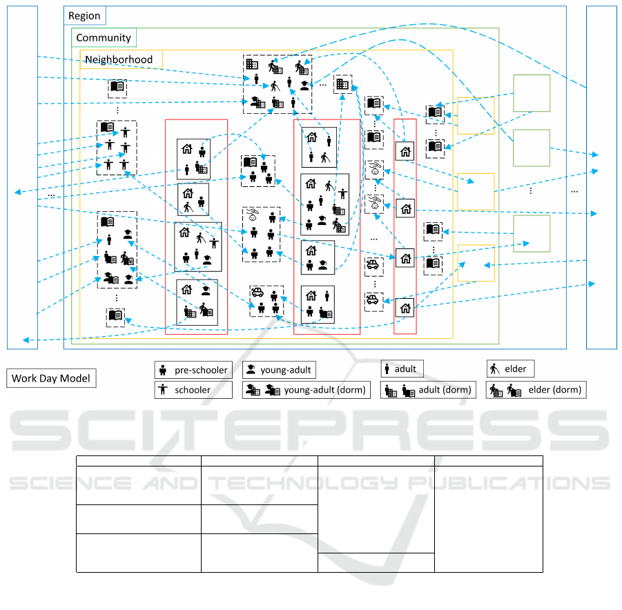
Figure 1: Schematic Chart of SimTW.

Table 2: Identities and holidays.

Identity Workday Holiday Long Holiday

Stay in home HH, CL, NB

home

, CM

home

Kindergartens KG, NB

home

, CM

home

Playgroup PG, NB

home

, CM

home

Daycare center DC, NB

home

, CM

home

Elementary school HH, CL, NB

home

, CM

home

Middle school SW, SC, NB

home

, CM

home

HH, CL, NB

home

, CM

home

High school

Commute university student UG, UC, NB

school

, CM

school

Commute worker WG, NB

work

, CM

work

Non-commute university student UG, UC, NB

school

, CM

school

UG, UC, NB

school

, CM

school

Non-commute worker WG, NB

work

, CM

work

WG, NB

work

, CM

work

3.1 Datasets

This work uses six different datasets to construct the

commute-related parameters. These datasets are cen-

sus data, household registration data, school data, na-

tional travel survey data, Google map data, and cal-

endar data. The relations between datasets and the

system conﬁgurations are shown in Figure 2.

3.1.1 Population Data

The census and household registration data are used

to build our system’s basic underlying social struc-

ture. The census and household registration data de-

tails are described in the previous work (Goh et al.,

2022). We here only mention those related to build-

ing the university and dormitory. In these datasets,

we use the age, the living and working location, and

the occupation to help us build the university and de-

termine the commuting type. The working location

has different recording granularities in Census 2000

and Census 2010. In Census 2000, we have the ex-

act region name of the working / studying location.

However, in Census 2010, the information on work-

ing locations only has three types:

1. Working and living in the same region;

2. Working and living in different regions but within

the same county (city);

3. Working and living in different counties (cities).

3.1.2 School Data

We collect data from Taiwan’s Ministry of Education

(MOE) (Department of Statistics, Ministry of Edu-

cation, R.O.C., ). According to the data, there were

SIMULTECH 2023 - 13th International Conference on Simulation and Modeling Methodologies, Technologies and Applications

306

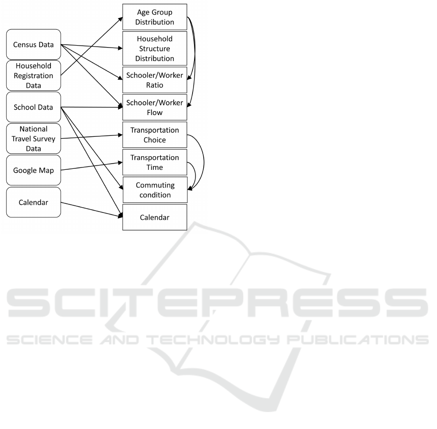
Figure 2: Dependency between data.

164 universities in the year 2010 in Taiwan. By using

the address of each school, we can determine each

school’s location (region). We also use the dormitory

status data to determine the dormitory size. Note that

from these data, we only know the number of students

at each university and the percentage of students who

chose to live in a dormitory. We need to ﬁnd out the

regions where those students come from.

3.1.3 Google Map Data

In order to determine the preference of a given agent,

who would like to commute every day or live in

a dormitory, we need to measure the transportation

distance between each region and the correspond-

ing transportation time. The Google Map API can

measure the transportation time between two regions.

Note that the transportation type affects the trans-

portation time a lot. The main difference is whether to

use the public transportation system or not. Using the

Google Map API, we get the transportation time from

region to region in different transportation types.

3.1.4 Transportation Data

We use the National Travel Survey data from

the Ministry of Transportation and Communications

(MOTC) (Department of Statistics, Ministry of Trans-

portation and Communications, R.O.C., ). National

Travel Survey data has been held every year since the

year 2009 but stopped from the year 2017 to the year

2019 and resumed in 2020. This survey data include

the gender, age, residential region, education level,

the most frequently used transportation means when

going out, whether the respondent went out yester-

day, the purpose and location of each activity the re-

spondent engaged in when the respondent went out all

day yesterday, the transportation means used and the

time spent, the reasons why people did not use public

transportation means, People’s satisfaction with us-

ing public transport and the reasons for their dissatis-

faction. There are 38,733 valid questionnaire survey

records in the year 2010.

By using the information of age, education level,

and purpose, we can separate the respondents into

university students or workers. This information

helps us to design different transportation strategies

for different identity agents. The preference for pub-

lic transportation or driving can differ for university

students and workers.

3.1.5 Calendar Data

We collected the calendar data from Taiwan’s

Directorate-General of Personnel Administration, Ex-

ecutive Yuan (Directorate-General of Personnel Ad-

ministration, Executive Yuan, Taiwan, ). The data

include workdays and holidays with types tagged.

Schools’ summer and winter vacations are collected

from each level of school. Note that the summer and

winter vacations are only valid for students. A day

has three types: workdays, holidays, and long holi-

days. Agents go to their workplaces and school dur-

ing the workdays. During the holiday, agents do not

go to work or school. When consecutive holidays

are longer than two days, they become long holidays.

During the usual holidays, agents who choose to com-

mute will stay in their homes, but those agents who

live in the dormitories stay in their dormitories. These

non-commute agents will return to their homes only

during the long holidays.

3.2 Constructing Commuting

Conﬁgurations

This subsection describes the conﬁgurations we need

to build the universities and dormitories. The ﬁrst is

the worker and student ﬂow tables; the second is the

probability table for determining the commuting type.

3.2.1 Constructing a Worker Flow Matrix

The worker ﬂow table W is a 368 × 368 matrix with

∑

W [i][[ j] = 1 for all i. Where 368 is the total number

of regions in Taiwan. Each W[i][ j] denotes the prob-

ability that an agent lives in region i has probability

Building Commuting Flows for an Agent Based Disease Spreading Simulation System Based on Aggregated Information

307

W [i][ j] to go to work in region j. By using the loca-

tion information from the census data, we construct

this table directly for the year 2000.

For 2010, we used the Census and household reg-

istration data information as the input constraints.

The input data shows the number of working adults

living in each region. We also know the number of

working adults that live but work in different regions.

Using this information, we can generate the region-

to-region working ﬂow and apply the maximum ﬂow

algorithm.

3.2.2 Constructing a University Student Flow

Matrix

The university student ﬂow table U is similar to the

worker ﬂow table, but it is a 368 × 164 matrix with

∑

U[i][ j] = 1 for all i. That is, this table gives the

probability that an agent lives in region i will have

probability U[i][ j] to go to university j. In order to

construct this table, we use the location information

from the census data and the size information from

the school data together. However, data from different

datasets have their own recording time and recording

errors. Therefore they can not use together directly.

By formulating the ﬂow table constructing problem as

a maximum ﬂow problem, we ﬁnd a maximum ran-

dom ﬂow to reduce the difference between different

datasets. The ﬂow problem can be seen as a two-stage

ﬂow problem. The ﬁrst stage is similar to the worker

ﬂow. That is the region-to-region student ﬂow. And

the second stage is a region to school ﬂow. That is, for

those students assigned to the same region, we need

to distribute them to different schools located in that

region.

3.2.3 Constructing Commuting Matrices

The commuting tables, C

, includes C

and C

are 368 × 368 0/1 matrices. When C

[i][ j] = 1

[i][ j] = 1), it means agents live in region i and

go to university (work) in region j prefers commuting

rather than live in a dormitory.

We use the following two different methods to

construct the C

matrices. The ﬁrst method uses the

traveling time and distance between each region pair.

According to the transportation data, we calculate the

average transportation time of each moving method.

We assume the university students may use the pub-

lic transportation system or drive themselves and can

tolerate a traveling time of up to 78 minutes. How-

ever, for the workers, the maximum traveling time for

going to work is usually less than 23 minutes.

The second method also considers the transporta-

tion survey data. According to the survey data, uni-

Table 3: Maximum tolerated time for the transportation.

Region Name

Worker Student

Public Drive Public Drive

New Taipei City 60 60 60 50

Yilan County 60 60 40 35

Taoyuan City 60 60 60 40

Hsinchu County 60 60 45 45

Miaoli County 60 60 50 38

Taichung County 60 60 50 40

Changhua County 60 60 50 40

Nantou County 60 60 50 45

Yunlin County 60 60 50 40

Chiayi County 60 60 50 30

Tainan County 60 60 50 30

Kaohsiung County 60 60 50 45

Pingtung County 60 60 50 30

Taitung County 60 60 50 25

Hualien County 60 60 50 30

Penghu County 60 60 50 20

Keelung City 60 60 50 60

Hsinchu City 60 60 50 30

Taichung City 60 60 50 40

Chiayi City 60 60 50 20

Tainan City 60 60 50 30

Taipei City 60 60 50 40

Kaohsiung City 60 60 50 40

Lienchiang County 60 60 50 5

Kinmen County 60 60 50 20

versity students and workers have different prefer-

ences when choosing moving methods and traveling

time. In this method, we ﬁrst determine whether an

agent prefers to take public transportation or drive it-

self. Next, we check whether the estimated traveling

time is larger or smaller than the tolerance threshold.

If the traveling time is less than the threshold, that

agent chooses to commute. Otherwise, that agent will

choose to live in a dormitory. Note that each region’s

public transportation system’s situation is different,

and each region’s tolerance threshold is also differ-

ent. Table 3 lists all the threshold times for workers

and students using different transportation methods in

each region. We construct two different C

matrices

using the above two methods.

4 EXPERIMENTS

4.1 Experiment Setting

In this section, we compare the following different

conﬁguration settings.

1. Mock populations with and without the universi-

ties.

2. Different tolerated threshold for transportation in-

formation.

SIMULTECH 2023 - 13th International Conference on Simulation and Modeling Methodologies, Technologies and Applications

308

Figure 3: Mock population with and without university and

dormitory.

We ﬁrst show the inﬂuence of having universi-

ties and dormitories. And then in the second exper-

iment, we show how the transportation preference af-

fects spreading of disease.

4.2 Experiment Result

4.2.1 Experiment with Universities and

Dormitories

Figure 3 compares the simulation result with and

without the university and dormitory. The line with

label v0.0 denotes the daily new infected cases in the

system without university and dormitory. The line

with label v2.0 denotes the daily new infected case in

the system with university and dormitory with com-

muting conﬁguration generated from Census 2000.

The line with label v2.1 denotes the daily new in-

fected case in the system with university and dor-

mitory with commuting conﬁguration generated from

Census 2010.

The experiment result shows that all three settings

have two local peaks under the same disease conﬁg-

uration. The two local peaks have nearly the same

height when there is no university. The cross-region

commuting is largely increased when there are uni-

versities and dormitories in the system. When we

add a dormitory into the system, the disease has a

lower spreading speed in the middle of the simula-

tion. Most university students stay in their dormito-

ries and only return home during the holidays. And

this also reduces the probability of university students

bringing the disease back to their hometown. When

the holidays come, the coming home university stu-

dents cause the second wave of infectious. The differ-

ence between the line v2.0 and v2.1 is the total num-

ber of university students. In 2010, the higher num-

ber of university students increased the height of the

ﬁrst peak in the simulation. This is because univer-

sity students are the main parts causing cross-region

transmission, and the second peak decreases due to a

lack of non-infected agents in the systems.

Figure 4: Different commuting conﬁguration for university

student and workers.

4.2.2 Experiment with Different Commuting

Conﬁguration

In Figure 4, we compare our system’s two commuting

conﬁgurations with the holiday conﬁguration. There

are three lines in the ﬁgure. The line with label v0.0

denotes the original baseline. The line with label v3.0

denotes the daily new infected case with the ﬁrst com-

muting conﬁguration with a long holiday setting. The

line with label v4.0 denotes the daily new infected

case with the second commuting conﬁguration with

a long holiday setting.

In the ﬁrst commuting conﬁguration, we have

a lower transportation tolerated threshold, mean-

ing most university students stay in the dormitories.

Therefore, the ﬁrst peak of this setting is much lower

than the other two and has a much higher second

peak. The second commuting conﬁguration has a

higher transportation tolerated threshold. Therefore

the fewer agents live in the dormitories, the higher the

ﬁrst peak is caused than the ﬁrst conﬁguration. No-

tice that the second conﬁguration also has a very high

and early second peak. This is because the amount

of non-commute people is much more than in the ﬁrst

conﬁguration.

5 CONCLUSION

In this work, we have shown how to build commut-

ing ﬂow in SimTW from the aggregated data. We

use the constrained-ﬂow algorithm to integrate differ-

ent datasets to generate the cross-region commuting

conﬁguration. From the experiment results, we have

found that the two main reasons affecting the disease

spreading are the amount of cross-region commut-

ing (commute or non-commute) and the daily activity

types (day type). With the newly added university and

dormitories components, detailed intervention strate-

gies can be designed and tested in our system to help

the domain experts design more speciﬁc public health

strategies.

Building Commuting Flows for an Agent Based Disease Spreading Simulation System Based on Aggregated Information

309

ACKNOWLEDGEMENTS

We thank Center for Survey Research (SRDA),

RCHSS, Academia Sinica, Taiwan for providing

data of Taiwan Census 2000 and 2010. This

study was supported in part by MOST, Taiwan

Grants 111-2221-E-001-017-MY3, 111-2221-E-033-

039 and 111-2634-FA49-014.

REFERENCES

Chang, H.-J., Chuang, J.-H., Fu, Y.-C., Hsu, T.-s., Hsueh,

C.-W., Tsai, S.-C., and Wang, D.-W. (2015). The im-

pact of household structures on pandemic inﬂuenza

vaccination priority. In SIMULTECH, pages 482–487.

Department of Statistics, Ministry of Education, R.O.C.

DOS, MOE, R.O.C. (Taiwan). Accessed: 2023-02-

20.

Department of Statistics, Ministry of Transportation and

Communications, R.O.C. DOS, MOTC, R.O.C. (Tai-

wan). Accessed: 2023-02-20.

Directorate-General of Personnel Administration, Execu-

tive Yuan, Taiwan. DGPA, R.O.C. (Taiwan). Ac-

cessed: 2023-02-20.

Geard, N., McCaw, J. M., Dorin, A., Korb, K. B., and

McVernon, J. (2013). Synthetic population dynam-

ics: A model of household demography. Journal of

Artiﬁcial Societies and Social Simulation, 16(1):8.

Germann, T. C., Kadau, K., Longini Jr, I. M., and Macken,

C. A. (2006). Mitigation strategies for pandemic in-

ﬂuenza in the united states. Proceedings of the Na-

tional Academy of Sciences, 103(15):5935–5940.

Goh, W.-P., Tsai, S.-C., Chang, H.-J., Lin, T.-Y., Chang, C.-

C., Pan, M.-L., Wang, D.-W., and Hsu, T.-s. (2022).

Household structure projection: A monte-carlo based

approach. In Proceedings of the 12th International

Conference on Simulation and Modeling Method-

ologies, Technologies and Applications (Simultech),

pages 70–79.

Lai, Z.-K., Chiang, Y.-T., Hsu, T.-s., and Chang, H.-J.

(2022). Using machine learning methods and the in-

ﬂuenza simulation system to explore the similarities of

taiwan’s administrative regions. In Proceedings of the

11th International Conference on Data Science, Tech-

nology and Applications, DATA 2022, Lisbon, Portu-

gal, July 11-13, 2022, pages 416–422.

Lin, C.-C., Ho, Y.-B., and Lin, Y.-L. (2011). An application

and the limitations of the census data for analyzing the

student sources of universities in taiwan. JOURNAL

OF GEOGRAPHICAL SCIENCE, 61.

Lin, T.-Y., Goh, W.-P., Chang, H.-J., Pan, M.-L., Tsai, S.-

C., Wang, D.-W., and Hsu, T.-s. (2021). Changing

of spreading dynamics for infectious diseases in an

aging society: A simulation case study on ﬂu pan-

demic. In 11th International Conference on Sim-

ulation and Modeling Methodologies, Technologies

and Applications, SIMULTECH 2021, pages 453–

460. SciTePress.

Tsai, M.-T., Chern, T.-C., Chuang, J.-H., Hsueh, C.-W.,

Kuo, H.-S., Liau, C.-J., Riley, S., Shen, B.-J., Shen,

C.-H., Wang, D.-W., and Hus, T.-s. (2010). Efﬁcient

simulation of the spatial transmission dynamics of in-

ﬂuenza. PloS one, 5(11):e13292.

Tsai, S.-C., Chen, C.-H., Shiao, Y.-T., Ciou, J.-S., and

Wu, T.-N. (2020). Precision education with statisti-

cal learning and deep learning: a case study in tai-

wan. International Journal of Educational Technol-

ogy in Higher Education, 17:1–13.

SIMULTECH 2023 - 13th International Conference on Simulation and Modeling Methodologies, Technologies and Applications

310