Analytical Model of Communication Algorithm for Simulations with

Range-Limited Interactions

Theresa Werner

, Christof P

aßler

, Ivo Kabadshow

and Matthias Werner

Department of Operating Systems, University of Technology Chemnitz, Germany

ulich Supercomputing Centre, Germany

Keywords:

Communication Algorithms, Time Analysis, Tradeoff Analysis, Range-Limited Interactions, Particle Simula-

tion.

Abstract:

With the development towards strong-scaling in High Performance Computing (HPC), many HPC applications

become communication-bound. One of them is the HPC Molecular Dynamics Simulation library FMSolvr,

which we are currently revising. In order to optimize communication, one could improve or develop new

communication protocols, but in this work we are focusing on problem-speciﬁc communication algorithms.

We found two promising candidates, the so-called Shift and what we call the Team Shift algorithm. In this

work we present an analytical model for the Shift algorithm and verify it. Our model is based on the Hockney

communication model and therefore only needs the two Hockney parameters α and β as input, so it can be

used on any network where the Hockney model is applicable.

1 INTRODUCTION

With the trend in High Performance Comput-

ing (HPC) towards strong-scaling, HPC programs

“ﬁnd their overall performance limited more by

performance of the communication network than

by the arithmetic performance of the nodes them-

selves (Hockney, 1994)”, i.e. HPC again became

communication-bound for many algorithms. Opti-

mizing communication hence has become a topic of

interest again. One way of optimizing is to work

on new communication protocols such as LCI (Dang

and Snir, 2018) or GASNet (Bonachea and Hargrove,

2018). Another way is to explore problem-speciﬁc

communication algorithms with less overhead. This

work focuses on the second approach.

We are interested in communication algorithms

that are suitable for Molecular Dynamics Simula-

tions (MDS). By conducting a Systematic Literature

Review on communication algorithms (Werner et al.,

2022) that might be suitable for our MDS library FM-

Solvr, we found two algorithms which are of inter-

est to us and may be of interest to scientists in other

ﬁelds of HPC, too. The two algorithms are Shift com-

munication as proposed by (Plimpton, 1995) and the

algorithm developed by (Driscoll et al., 2013) that is

based on the Shift and will be referred to as Team Shift

because it uses processor teams. Seeing that the two

algorithms seem to be suitable for covering different

ranges in the context of range-limited interactions –

Shift covering smaller areas than Team Shift – there

must be one or more tradeoff points where the Team

Shift starts to outperform the Shift.

In this work, we present an analytical model for

the ﬁrst algorithm, the Shift. We start with the Shift

because it has higher relevance for FMSolvr due to

being optimal for covering small ranges. With an im-

plementation of the Shift algorithm, we can show that

the Shift model can predict the real timing behavior

of the implementation and hence can be used to ﬁnd

the tradeoff points once we have a Team Shift model

as well. The only precondition for our model is deter-

mining the Hockney (Hockney and Jesshope, 1988)

model parameters α and β, which can be determined

by “ping pong” measurements.

Once we have a veriﬁed Team Shift model as well,

revised FMSolvr will be able to select its communi-

cation algorithm by only being given the Hockney pa-

rameters of the target system as input.

As for the structure of this work: Section 2 in-

troduces the reader to the two communication algo-

rithms; Section 3 walks the reader through the analyt-

ical model of the Shift; Section 4 gives insight into

our system properties and implementation speciﬁcs

and explains how to determine the Hockney param-

eters for a given system; Section 5 compares the Shift

Werner, T., PÃd’Ã§ler, C., Kabadshow, I. and Werner, M.

Analytical Model of Communication Algorithm for Simulations with Range-Limited Interactions.

DOI: 10.5220/0012085500003546

In Proceedings of the 13th International Conference on Simulation and Modeling Methodologies, Technologies and Applications (SIMULTECH 2023), pages 311-317

ISBN: 978-989-758-668-2; ISSN: 2184-2841

 2023 by SCITEPRESS – Science and Technology Publications, Lda. Under CC license (CC BY-NC-ND 4.0)

311

model predictions to the measurements of the imple-

mentation; and Section 6 summarizes this work, dis-

cusses certain details, and gives an outlook to future

work.

2 ALGORITHM DESCRIPTION

2.1 Problem Description

Before we look at the two algorithms, we should look

at the problem they were developed for. Without go-

ing too deep into the physics of MDS, the scenario

can be described as follows: we cut our simulation

space (our particle system) into same-sized cubes or

boxes in order to distribute the work over the compu-

tation nodes. Every compute node holds one of these

boxes

. Each box contains a subset of particles of the

particle system. This subset of particles interacts with

itself but also with particles of boxes that are handled

by other nodes. So, in order to simulate the move-

ment of its subset of particles properly, a node must

exchange data with all nodes that hold boxes which

are neighboring boxes of its own box, i.e. the data

from other nodes must be transferred over the net-

work. Figure 1 illustrates the problem for the dark

blue and the dark orange box in a two-dimensional

simulation space.

In a three-dimensional simulation, one node has

a total of (2k + 1)

− 1 exchange partners where k ∈

N stands for the layers of neighbors around the box,

aka. cut-off radius. Parameter k = 1 means the ﬁrst

layer of neighbors, which share a face, an edge, or a

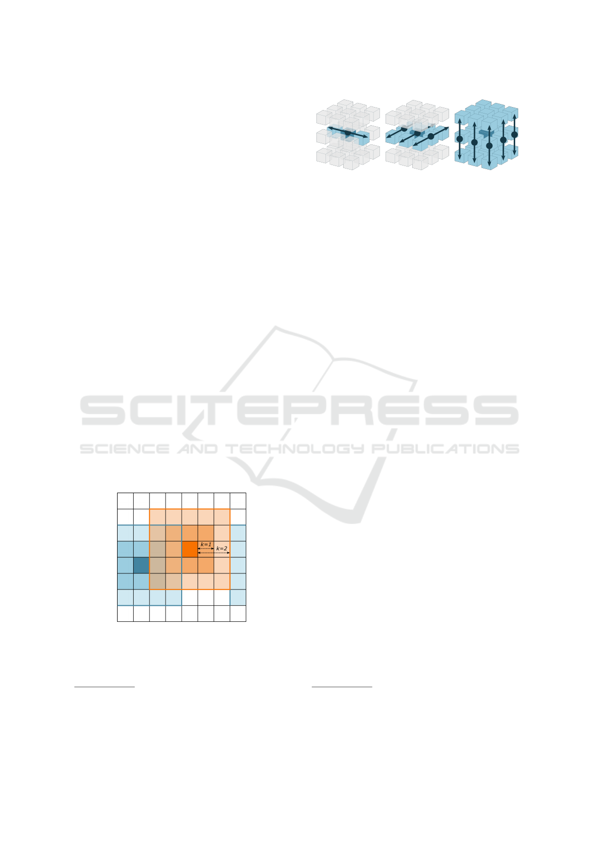
Figure 1: Neighbors of a box. Each node requires the data

of boxes that are neighbors to its own box. The neighbors of

the dark orange box are light orange; the neighbors of the

dark blue box are light blue. Boxes may share neighbors.

The size of the neighborhood is deﬁned by k ∈ N.

In fact, a node may hold several boxes, but for sim-

plicity we shall consider the case of one box per node. An

algorithm for multiple boxes per node is described in (Liem

et al., 1991), which is an early version of the Shift.

(a) (b) (c)

Figure 2: Shift by (Plimpton, 1995). First, the data is dis-

tributed along the row. Then, the accumulated row data is

distributed along the column. Last, the accumulated data

of the plane is distributed within the tower (vertical dimen-

sion).

corner with the center box; k = 2 means the second

layer of neighbors, which share a face, an edge, or a

corner with the ﬁrst-layer neighbors. For Figure 1 k is

two. So, how do we reduce the number of (2k +1)

−

1 point-to-point messages and make communication

more efﬁcient?

2.2 Classic Shift Communication

The Shift communication algorithm uses proxy com-

munication to reduce the number of messages. What

is meant by proxy? Every node only communicates

with its six direct logical

neighbors Left, Right,

Front, Back, Up, and Down. If a node needs to ex-

change data with a node that is not one of the six direct

logical neighbors, its neighbors take care of daisy-

chaining the data to its destined receiver. In order to

allow this proxy behavior with only six neighbors and

still get the data to all relevant places the nodes must

follow a special communication pattern.

Figure 2 illustrates the three phases of the Shift:

ﬁrst, a node sends its data to its Left and Right neigh-

bor and receives their data in return (see Fig. 2a). If

k > 1, the node will now send the data it received

from the Left neighbor to its Right neighbor and vice

versa. In return, it receives the data of its second next

neighbors to the right and left. This continues until

all nodes within one row have all the data of nodes

k positions up and down the row. Second, the row

data is pooled into one message and sent to the Front

and Back neighbor (see Fig. 2b). Equivalent to the

procedure in the row, the data packages are daisy-

chained along the column for k > 1. Third, the data

of the plane is combined into one message and sent

to the Up and Down neighbors along what we call the

towers (see Fig. 2c). That concludes the classic Shift

communication by (Plimpton, 1995).

A neighbor in this context does not mean a physical

neighbor, but a node that holds the neighboring box to the

node’s own box. In any ﬁgure, we assume the logical neigh-

bors to be physical neighbors.

SIMULTECH 2023 - 13th International Conference on Simulation and Modeling Methodologies, Technologies and Applications

312

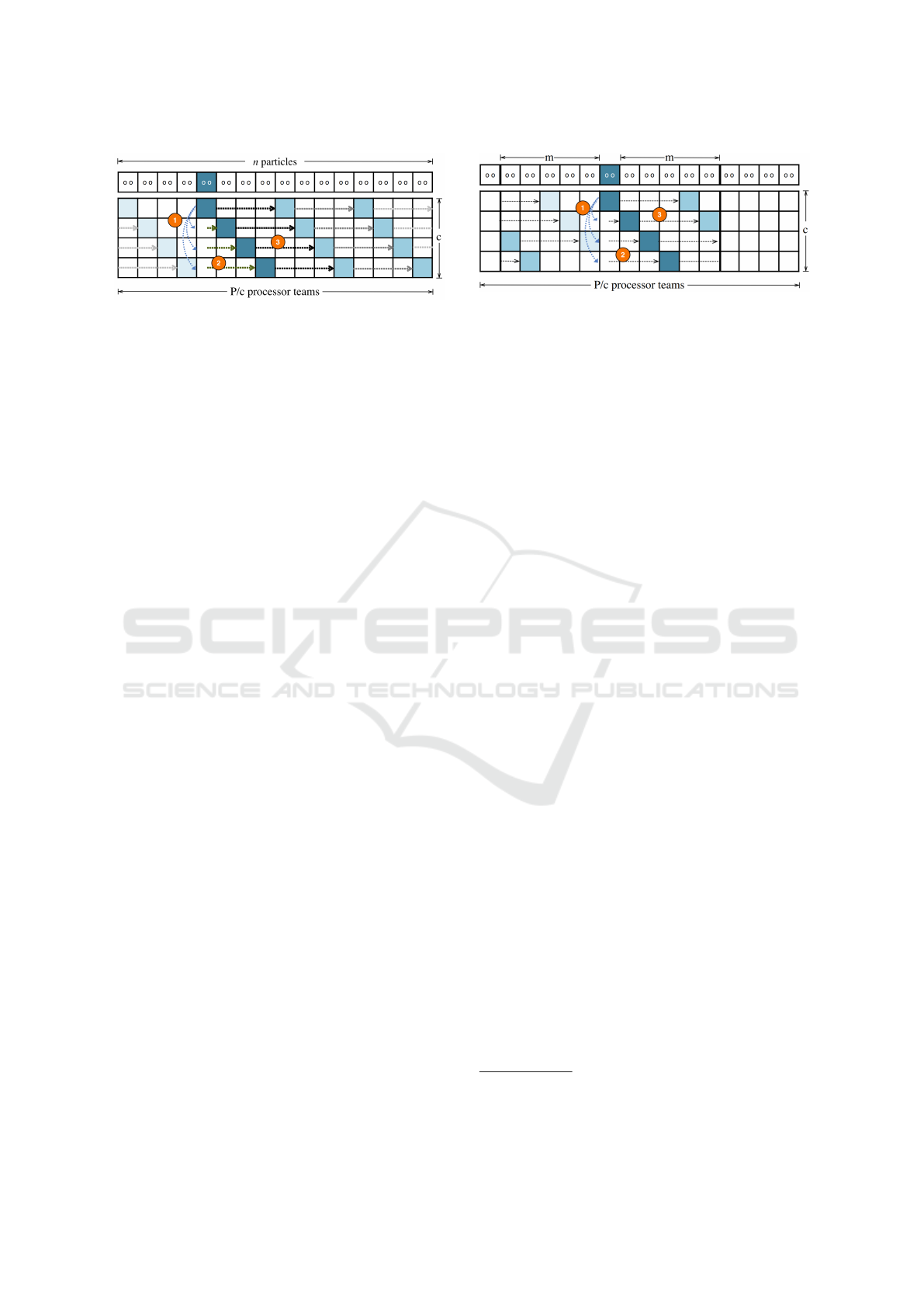
Figure 3: Team algorithm by (Driscoll et al., 2013). First,

the data is distributed within the team. Second, the data

is “tilted” among the teams. Third, the data is shifted in a

wrap-around fashion around the whole space. Last, the ac-

cumulated data of each team is gathered by the team leader.

(Graphic from (Driscoll et al., 2013).).

2.3 Team Shift Communication

The Team Shift communication algorithm was orig-

inally developed for an all-to-all exchange between

nodes instead of a local interaction set. The method

can, however, be adjusted to our application. But let

us look at the original algorithm ﬁrst, which is dis-

played in Figure 3.

The algorithm uses three important parameters:

the total number of processors P, the number of mem-

bers in a team c (for copy), and the resulting num-

ber of teams T = P/c. The data (represented by tiny

circles in Fig. 3) is distributed evenly over the teams

without regard for order or spatial context. The team

leader broadcasts the data within its team (step

⃝).

Next, the data is “tilted” among the teams (step

⃝).

Then, every team member daisy-chains (step

⃝) the

received data from a dedicated sender, which is c

teams up the row, to a dedicated receiver, which is

c teams down the row. This is done until the data

has circled once all around the teams (wrap-around).

Last, the team leader gathers the data its team mem-

bers have accumulated, which is all the data of all

teams.

Step

⃝ has the effect that a team has data of c

different teams before it starts daisy-chaining data in

step

⃝ like in the Shift algorithm. This allows to

daisy-chain/shift in steps of c, i.e. to cover a much

bigger distance in one shift than is possible with the

Shift algorithm.

(Driscoll et al., 2013) extended this algorithm to

ﬁt the problem of a local interaction set. This time

the data is distributed with regard to spatial context,

i.e. the simulation space is cut and distributed like for

the Shift. And they constrained the global algorithm

to wrap around the distance deﬁned by m (their m is

our k), see Figure 4. The Team Shift with only one

team member is almost identical to the Shift. The only

exception is that data is daisy-chained only in one di-

Figure 4: Team Shift by (Driscoll et al., 2013). Instead

of wrapping around the whole space, the algorithm wraps

around the cut-off area deﬁned by m (their m is our k).

(Graphic from (Driscoll et al., 2013).).

rection and wrapped around the cut-off k instead of

being daisy-chained in both directions.

While the all-to-all algorithm can simply line up

all boxes and wrap around this single dimension, the

range-limited algorithm must be performed thrice,

once into each dimension, because we now have spa-

tial context and not a random distribution of particle

data.

3 COMMUNICATION MODEL

3.1 Hockney Model

We are using what is commonly known as the Hock-

ney (Hockney and Jesshope, 1988, pp.85) model or

the “postal” model of communication

because de-

spite its simplicity it is able to make accurate pre-

dictions about message latency and focuses solely on

the communication and not on computation or other

aspects of the machine. The PRAM (Fortune and

Wyllie, 1978) model is not suitable for us since it

mainly focuses on shared memory machines, and the

BSP (Valiant, 1990) and LogP (Culler et al., 1993)

models only use an upper bound for latency instead

of calculating an accurate latency value; as the Shift

(and Team Shift) works with increasing message load

in different stages of the algorithm, an upper bound

for latency is not useful for us. Also, the o and g pa-

rameter of the LogP model are too sophisticated for

our purposes, and the effort of determining these pa-

rameters is disproportionate compared to the expected

gains.

In the Hockney model each message consists of

a constant part α, which represents the latency of an

empty message, and the variable part β · m where β

represents the inverse bandwidth (time per byte) and

The original model is slightly more complex, but the

reduced model we are using is commonly used and sufﬁ-

cient for our purpose.

Analytical Model of Communication Algorithm for Simulations with Range-Limited Interactions

313

m the number of bytes in the message. Together this

makes a total message time of

T = α + β · m .

3.2 Shift Model

For the Shift each node must send k messages into

each direction, and each message takes the time

α + βm

, where m

is the message size depending on

the dimension/phase. Thus, for each dimension we

spend a total time of

= 2k · (α + β · m

) . (1)

The message size for the exchange within the row is

. The message content of the next dimension com-

prises of the k messages of the right neighbors, the

k messages of the left neighbors, and the node’s own

data, so 2k + 1 message contents of the previous di-

mension. Therefor, he message size for the column

dimension is

= (2k + 1) · m

and the message size for the tower dimension is

= (2k + 1) · m

= (4k

+ 4k + 1) · m

So, we get an overall communication time of

Shift

= 6k · α + 2k · β(m

+ m

)

= 6k · α + β · m

(8k

+ 12k

+ 6k) .

(2)

If, like in our case, a node cannot send and receive at

the same time (see Sec. 4.1), each exchange consists

of two consecutive sending processes instead of two

concurrent ones, so Equation 2 must be multiplied by

two. Hence, we get

Shift

= 12k · α + 2β · m

(8k

+ 12k

+ 6k) .

(3)

4 METHODS

4.1 Implementation Background

Our cluster JURECA has an InﬁniBand network with

MPI (we used OpenMPI 4.1.2). MPI has two differ-

ent modes of sending, eager and rendezvous proto-

col. Eager protocol is for small messages (< 256kB

The send call returns immediately because the re-

ceiver is known to have enough buffer to receive the

message. For message sizes above that limit, MPI

uses the rendezvous protocol, which means that the

The limit is supposed to be much lower, but we mea-

sured it at 256kB.

Figure 5: Coordinating communication with MPI Ssend:

First, the blue ranks send their data and the orange ranks

receive, then the orange ranks send their data and the blue

ranks receive.

sending node performs a handshake with the receiv-

ing node to make sure that the other is ready to re-

ceive the message and prepare its buffers accordingly.

Eager protocol causes different behavior on sending

and receiving nodes, which we want to avoid for now.

Hence, we use MPI_Ssend, the synchronized version

of the MPI_Send that forces a rendezvous. Due to this

constraint a node cannot send and receive at the same

time.

4.2 Implementation Details

For verifying our model we only implemented one di-

mension of the Shift algorithm (distribution in row).

Since all three dimensions use the exact same al-

gorithm only with a difference in message size,

we can safely assume that if we verify the one-

dimensional model with different message sizes, the

three-dimensional model is valid as well (small over-

head for repackaging not considered).

Since every node receives the same number of

data elements, each node knows the number of data

elements each other node holds. From this informa-

tion and the given cutoff radius k, one can extract the

number of data elements that will be received during

the course of the algorithm. The buffer is then al-

located to ﬁt 2k + 1 messages. Each node places its

own data in the middle of the buffer (buffer[k]).

The data it receives will be ﬁlled into the buffer

sorted by origin. The data of the Right neighbor

will be ﬁlled into the next buffer spot after the own

data (buffer[k+1]) and the data of the Left neigh-

bor into the spot before the own data (buffer[k-1]),

then the data of the second-next neighbors into

buffer[k+2] and buffer[k-2], and so on. This

helps with ﬁnding the matching data for every mes-

sage.

To ensure correctness of the algorithm, we send

test data with each message. So, each node’s buffer

space is ﬁlled with test data to check results later, the

rest of the communication buffer is cleared. Then,

all processors are synchronized via MPI_Barrier and

the time measurement begins.

The ranks a node communicates with are calcu-

lated with modulo arithmetic to ensure correct behav-

ior at the ends of the communicator (we have peri-

SIMULTECH 2023 - 13th International Conference on Simulation and Modeling Methodologies, Technologies and Applications

314

odic boundary conditions for the simulation space).

A node, before sending or receiving a message, calcu-

lates the rank of the real source of the next incoming

and outgoing message in order to place it in or retrieve

it from the correct spot in the message buffer.

Due to the use of MPI_Ssend, we need to assure

that no deadlocks will occur (e.g. two nodes posting a

receive call for each other). To avoid that, we use an

even-odd-pattern for the communication, where the

nodes with an even rank are depicted in blue and those

with an uneven rank are depicted in orange (for visu-

alization see Fig. 5). In the ﬁrst step, each blue node

sends its message while the orange nodes receive the

messages; in the second step, the roles swap and the

orange nodes become senders while the blue ones re-

ceive the messages. Since we used 64 nodes, we did

not need to consider an extra phase for the case of two

blue nodes meeting at the edges of the row.

Further, we dictate a sequence for the communica-

tion: ﬁrst we daisy-chain all right messages k times,

then we daisy-chain all left messages k times. An-

other way would be to interleave the right and left

messages.

After all of the 2k messages have been exchanged,

the measurement ends and the message buffers are

checked for correctness.

4.3 Implementation Measurements

We used 64 nodes and ran the algorithm 100 times

for each cut-off k ∈ [1, 10]. This resulted in 6400 data

elements per k-value. So, all measured values pre-

sented in this work are averaged over 6336 measure-

ments (the ﬁrst measurement of each node is excluded

because it is 100 times slower than the rest due to the

path routing process).

4.4 Hockney Parameters

As (Lastovetsky et al., 2009) wrote in their paper, the

Hockney parameters α and β are typically estimated

by statistically evaluating one of two series of point-

to-point communications:

• Roundtrips between two nodes with an empty

message to determine α and roundtrips between

two nodes for each relevant message load to de-

termine β with respect to m.

• A series of roundtrips with a growing message

load, so that a linear regression can be ﬁtted over

the resulting curve.

Some of our messages are too small to show a linear

relation (messages <50kB), so we used the ﬁrst op-

tion for our measurements. To make sure that we do

Table 1: Message latency in relation to message load with

derived Hockney parameter β.

load [byte] latency [ns] σ [ns] β [ns/byte]

0 2,122 176 –

10 2,234 183 11.246

100 2,686 302 5.645

1,000 2,881 305 0.760

10,000 4,808 307 0.269

100,000 15,055 749 0.129

not have different latencies between node pairs due

to varying physical distance of nodes, we measured

the latency between nodes from different racks. After

making sure that we have sufﬁcient location invari-

ance (physical distance has no measurable inﬂuence

on the latency), we gathered data over several days

with a morning and an afternoon measurement with a

set of four random nodes each time (to account for dif-

ferent network load patterns of other users that might

inﬂuence our model negatively).

We used a one-to-all ping pong from the node with

MPI rank zero to the three other nodes of the set. For

each pair we returned for every value m

the average

over 10,000 roundtrips. Overall, we performed ten

measurements, getting thirty sets of data per m

-value

per measurement, so 300 data elements for each mes-

sage load value m

We determined the Hockney parameters by using

the average over all 300 data elements per m

-value.

Table 1 shows the average latency by load m

and

the derived β (standard deviation σ over 300 data ele-

ments); the latency value for zero bytes is used for α.

5 SHIFT MODEL ANALYSIS

We explained in Section 4.2 that we implemented

only one dimension/phase of the Shift, so we use

Equation 1 multiplied by two to predict the timing be-

havior for the Shift in the row dimension.

Table 2 shows one representative example of

the measurements and predictions for the one-

dimensional Shift algorithm with the respective stan-

dard deviation σ for the measurements; tables for the

other message loads can be found in the Appendix.

The data in Tables 2 to 6 shows that the model

works very well for message loads m

of 10 to

1,000 bytes but becomes less accurate for larger m

However, our predictions are within the stan-

dard deviation of the measurements for all message

loads (10 to 100,000 bytes), hence our model can be

considered correct.

Analytical Model of Communication Algorithm for Simulations with Range-Limited Interactions

315

Table 2: Shift (1D) with m

= 1, 000 bytes.

k measured predicted

latency [ns] σ [ns] latency [ns]

1 13,804 5,294 11,526

2 22,494 3,715 23,051

3 34,814 6,499 34,577

4 45,422 8,145 46,103

5 55,957 11,090 57,628

6 68,121 20,231 69,154

7 78,428 15,781 80,679

8 93,194 21,057 92,205

9 102,293 18,898 103,731

10 114,216 20,178 115,256

6 CONCLUSION

6.1 Summary

We want to model two communication algorithms,

Shift by (Plimpton, 1995) and Team Shift by (Driscoll

et al., 2013), in order to equip out MDS library FM-

Solvr with an adaptive communication module that

can choose the communication algorithm based on the

hard- and middleware of the underlying system (re-

spective the α and β of the Hockney model).

In this work we present an analytical model for

the Shift communication algorithm and veriﬁed it by

implementation.

6.2 Discussion and Future Work

6.2.1 Implementation

We imposed certain constraints upon our system (see

Sec. 4.1 and 4.2), which we will relax on our way to a

realistic performance model. Our strongest constraint

is that we forced the synchronous rendezvous on our

system by using MPI_Ssend. This constraint has to

be relaxed in order to beneﬁt from using MPI_Send or

even MPI_Isend and get a more efﬁcient implemen-

tation.

By using MPI_Ssend or MPI_Send we are forced

to dictate a pre-deﬁned pattern for the communication

by sending ﬁrst all messages to the right, then all mes-

sages to the left. The Shift algorithm allows for self-

synchronization, so once we allow using MPI_Isend

we are able to let go of the constricting rules of where

to send ﬁrst and can decide the next message based on

which data is already available.

6.2.2 Hockney Parameters

As we already concluded in Section 5, the data in

Tables 2 to 6 shows that the model works very well

for m

∈ [10,1000] bytes but becomes less accurate

for larger m

. We can also see that the latencies for

the three smaller m

show barely any difference (not

even 20 µs between 10 and 1,000 bytes for k = 10)

while the difference increases to almost twice the

amount of time between 1,000 and 10,000 bytes and

again to about thrice the time between 10,000 and

100,000 bytes.

We think that the inaccuracy of the model for

larger m

might be because the Shift algorithm is

causing a lot of trafﬁc in the network which becomes

noticeable once the message size starts to saturate the

bandwidth more. However, a single ping pong mea-

surement does not create its own background trafﬁc.

Our approach is to re-measure α and β while creating

a lot of trafﬁc in the background so as to simulate the

algorithm limiting itself.

6.2.3 Data Analysis

Since our data has not been ﬁltered apart from drop-

ping the ﬁrst measurement of each node, we can see

in Tables 2 to 6 that our standard deviation is com-

parably high (a sign for noisy measurements). In a

few cases so much so that it makes the usefulness of

the resulting average questionable (m = 10,000 bytes,

k ∈ {2,9}, and m = 100,000 bytes, k ∈ {6,8}).

One approach we tried was to use only the 20%

smallest values with the argument that we are inter-

ested in the best case anyway and everything above

that is inﬂuenced by network noise. This must re-

ﬂect in the α- and β-values too, so we excluded the

higher values in the α and β measurements. This ap-

proach delivers extremely good standard deviations of

less than 2 µs (in most cases even less than 1 µs, and

in very few cases for 10,000 and 100,000 bytes up to

4 µs) and makes the model an almost perfect ﬁt for the

measurements.

However, we did not ﬁlter α and β systematically

for the smallest 20% and we cannot give a more justi-

ﬁed reason behind the selected 20% margin other than

trial-and-error evaluation. Future work will be to re-

evaluate all data in this fashion systematically.

6.2.4 Analytical Models

A comprehensive complexity analysis is not part of

this work since it is trivial in case of the Shift algo-

rithm.

The model already is a non-rendezvous version,

i.e. a version where a node can send and receive at the

same time, so it should be able to model an implemen-

tation with MPI_Send or MPI_Isend. After looking at

the future work proposed in 6.2.2 and 6.2.3, we will

measure these implementations next. Then we will

look at the model for the Team Shift.

SIMULTECH 2023 - 13th International Conference on Simulation and Modeling Methodologies, Technologies and Applications

316

ACKNOWLEDGMENTS

This research is funded by DFG project FMHub,

project Nr. 443189148. Our thanks goes to Andreas

Beckmann

and Martin Richter

for helping with the

implementation and evaluation respectively.

REFERENCES

Bonachea, D. and Hargrove, P. (2018). GASNet-EX: A

High-Performance, Portable Communication Library

for Exascale. In Proceedings of Languages and Com-

pilers for Parallel Computing (LCPC’18).

Culler, D., Karp, R., Patterson, D., Sahay, A., Schauser,

K. E., Santos, E., Subramonian, R., and Von Eicken,

T. (1993). LogP: Towards a realistic model of paral-

lel computation. In Proceedings of the fourth ACM

SIGPLAN symposium on Principles and practice of

parallel programming, pages 1–12.

Dang, H.-V. and Snir, M. (2018). LCI: Low-level communi-

cation interface for asynchronous distributed-memory

task model. In ACM Conference (Conference’17).

Driscoll, M., Georganas, E., Koanantakool, P., Solomonik,

E., and Yelick, K. (2013). A Communication-Optimal

N-Body Algorithm for Direct Interactions. In 2013

IEEE 27th International Symposium on Parallel and

Distributed Processing, pages 1075–1084.

Fortune, S. and Wyllie, J. (1978). Parallelism in random

access machines. In Proceedings of the tenth annual

ACM symposium on Theory of computing, pages 114–

118.

Hockney, R. W. (1994). The communication challenge for

MPP: Intel Paragon and Meiko CS-2. Parallel Com-

puting, 20(3):389–398.

Hockney, R. W. and Jesshope, C. R. (1988). Parallel Com-

puters 2: architecture, programming and algorithms.

IOP Publishing Ltd.

Lastovetsky, A., Rychkov, V., and O’Flynn, M. (2009). Re-

visiting communication performance models for com-

putational clusters. In 2009 IEEE International Sym-

posium on Parallel & Distributed Processing, pages

1–11. IEEE.

Liem, S. Y., Brown, D., and Clarke, J. H. R. (1991).

Molecular dynamics simulations on distributed mem-

ory machines. Computer Physics Communications,

67(2):261–267.

Plimpton, S. (1995). Fast Parallel Algorithms for Short-

Range Molecular Dynamics. Journal of Computa-

tional Physics, 117(1):1–19.

Valiant, L. G. (1990). A bridging model for parallel compu-

tation. Communications of the ACM, 33(8):103–111.

Werner, T., Kabadshow, I., and Werner, M. (2022). System-

atic Literature Review of Data Exchange Strategies for

Range-limited Particle Interactions. In Proceedings of

the 12th International Conference on Simulation and

Modeling Methodologies, Technologies and Applica-

tions, pages 218–225.

APPENDIX

Table 3: Shift (1D) with m

= 10 bytes.

k measured predicted

latency [ns] σ [ns] latency [ns]

1 11,360 4,332 8,937

2 19,478 1,765 17,873

3 30,071 8,554 26,810

4 39,338 11,080 35,746

5 48,424 10,598 44,683

6 58,701 16,412 53,619

7 66,476 9,267 62,556

8 75,920 10,316 71,492

9 88,762 24,108 80,429

10 97,072 25,594 89,366

Table 4: Shift (1D) with m

= 100 bytes.

k measured predicted

latency [ns] σ [ns] latency [ns]

1 12,108 3,489 10,745

2 21,388 4,860 21,489

3 32,193 5,712 32,234

4 41,966 6,732 42,978

5 52,296 11,298 53,723

6 62,299 10,229 64,467

7 73,683 14,560 75,212

8 84,488 23,172 85,956

9 91,207 15,943 96,701

10 101,664 15,741 107,446

Table 5: Shift (1D) with m

= 10, 000 bytes.

k measured predicted

latency [ns] σ [ns] latency [ns]

1 21,925 7,736 19,233

2 49,498 52,127 38,465

3 65,985 29,351 57,698

4 82,636 18,911 76,931

5 102,159 21,077 96,163

6 121,945 20,153 115,396

7 143,613 38,003 134,629

8 164,761 38,274 153,861

9 198,848 86,793 173,094

10 207,388 52,577 192,327

Table 6: Shift (1D) with m

= 100, 000 bytes.

k measured predicted

latency [ns] σ [ns] latency [ns]

1 62,708 7,353 60,219

2 127,668 19,557 120,438

3 191,647 29,054 180,657

4 263,956 65,629 240,877

5 319,701 65,497 301,096

6 467,980 492,450 361,315

7 448,284 83,874 421,534

8 565,866 389,992 481,753

9 585,111 109,965 541,972

10 671,048 169,343 602,192

Analytical Model of Communication Algorithm for Simulations with Range-Limited Interactions

317