Real Time Orbital Object Recognition for Optical Space Surveillance

Applications

Radu Danescu

, Attila Fuzes

, Razvan Itu

and Vlad Turcu

Computer Science Department, Technical University of Cluj-Napoca, Memorandumului 28, Cluj-Napoca, Romania

Astronomical Observatory Cluj-Napoca, Romanian Academy, Ciresilor 19, Cluj-Napoca, Romania

Keywords: Space Surveillance, Real Time Target Identification, Low Earth Orbit.

Abstract: Artificial objects in various orbits surround the Earth, and many of these objects can be found within the low

Earth orbit region (LEO). This orbital zone also contains a significant amount of space debris, which pose a

tangible threat to space operations, necessitating close monitoring. Various sensors can be used for either

tracking, knowing the target’s orbital parameters and observing it for updating them, or for surveillance, which

can also discover new targets. Real time identification of the satellite as it is detected by the surveillance

systems provides a mechanism for selecting the targets for stare and chase applications, to decide if a new

satellite has been discovered, or to identify a satellite that has outdated orbital elements. This paper describes

a system capable of real time surveillance and satellite identification using limited computing power. The

system relies on detecting trajectory endpoints at discrete time intervals, and then using these endpoints for

frame by frame trajectory prediction, which is then matched with detected tracklets. This way, the tracklets

are identified in real time. The system has been tested by surveying real satellites, in real time, and the

identification mechanism proved to work as expected.

1 INTRODUCTION

Artificial objects in various orbits surround the Earth,

and many of these objects can be found within the low

Earth orbit region (LEO), typically at altitudes below

2000 km. Besides useful satellites, this orbital zone

contains space debris, which pose a tangible threat to

space operations, necessitating close monitoring.

Many of the LEO satellites’ orbital parameters are

stored in the Space-Track catalogue (SpaceTrack,

2023), which is maintained by the Space Fence Radar

system (Haimerl, 2015, and LockheedMartin, 2022).

While the radar sensors are highly accurate and

can track small objects even in adverse weather

conditions, they are expensive to set up and operate.

Optical sensors, on the other hand, are cheaper, have

a highly accurate angular resolution, and can be easily

deployed all over the world. The sensor can be used

either for tracking, knowing the target’s orbital

parameters and observing it for updating them, or for

surveillance, which can also discover new targets.

https://orcid.org/0000-0002-4515-8114

https://orcid.org/0000-0001-8156-7313

The sensors used for tracking have narrow fields of

view (FOV) and large focal lengths, while the sensors

used for surveillance have wider field of view and

shorter focal lengths.

Some algorithms rely on a priori knowing the

expected trajectory of the satellite, such as the

approach presented in (Levesque, 2007), which relies

on background modelling and subtraction using a

polynomial intensity model, combined with star

removal and matched filters for streak detection, or a

similar approach, presented in (Vananti, 2015),

employs background modelling and subtraction, and

convolution with shaped kernels for streak detection.

When the trajectory is not known, the algorithms

try to detect generic linear shapes in the image. Such

generic structures can be detected using the Radon

transform, which can be combined with matched

filters, as in (Hickson, 2018), or combined with an

intensity profile along the emphasized line (Ciurte,

2014). The linear shape of the streak can be

highlighted also by the Hough transform, a popular

562

Danescu, R., Fuzes, A., Itu, R. and Turcu, V.

Real Time Orbital Object Recognition for Optical Space Surveillance Applications.

DOI: 10.5220/0012158800003543

In Proceedings of the 20th International Conference on Informatics in Control, Automation and Robotics (ICINCO 2023) - Volume 1, pages 562-569

ISBN: 978-989-758-670-5; ISSN: 2184-2809

line matching technique. This approach is used in

(Wijnen, 2019) and in (Diprima, 2018), where it is

combined with morphological operations. RANSAC,

a method for stochastic fitting of lines, was also used

in combination with the Hough transform by (Wijnen,

2019). The streaks can also be identified through

thresholding and connected components analysis for

specific geometric properties, as in (Virtanen, 2016),

(Kim, 2016). Another characteristic of the satellite

streaks is that they tend to have a colinear trajectory in

successive frames. This property can be used for

increasing the accuracy and robustness of the results,

as shown in (Do, 2019) and (Danescu, 2022).

The algorithms can be used with specialized

systems set up on vast areas all over the world, such

as TAROT (Boer, 2017), a network of fast acting

telescopes distributed worldwide and coordinated by

France, the OWL Net network (Park, 2018), a South

Korea coordinated array of telescopes offering fully

robotic operation for observing LEO and GEO orbits

with high accuracy, or the FireOpal network (Bland,

2018), which consists of multiple all sky observation

stations in the Australian desert, equipped with on-

site image processing and astrometric reduction

capabilities.

As alternatives to complex and centralized

solutions, low-cost solutions that can be easily set up

anywhere are presented in (Langbroek, 2023) and

(Danescu, 2022). As shown in (Langbroek, 2023), an

informal network of low-cost systems can be used to

discover and track objects that are not found in

official catalogues, and informal catalogues of

classified objects can be maintained (McCants,

2023).

The surveillance systems can discover new

satellites, or can adjust the parameters of satellites that

have outdated parameters, such as those that will soon

re-enter the atmosphere. Real time capabilities for

detection and identification are essential in these types

of applications. The accuracy of the surveillance

process can be enhanced by combining the detection

power of the wide FOV systems with the accuracy of

the telescopes using the “stare and chase” strategy.

The initial wide FOV detection will be used for short

time trajectory prediction, and a telescope will be

locked in for precise tracking (Hasenohr, 2016),

(Danescu, 2023).

Real time identification of the satellite as it is

detected by the surveillance system is valuable, as it

provides a mechanism for selecting the target in stare

and chase applications, to decide if a new satellite has

been discovered, or to identify a satellite that has

outdated orbital elements. This paper describes a

system capable of real time surveillance and satellite

identification using limited computing power. The

system relies on detecting trajectory endpoints at

discrete time intervals, and then using these endpoints

for frame-by-frame trajectory prediction, which is

then matched with detected tracklets. This way, the

tracklets are identified in real time.

2 SOLUTION OVERVIEW

The real time detection and recognition system runs

three processes in parallel, as shown in Figure 1. The

detection process handles every newly acquired

image, detects the moving streak-like structures, and

connects them into tracklets (sequences of detected

streak positions).

The calibration process runs the automatic star

identification methods provided by Astrometry.net

(Lang, 2010), and generates calibration parameters

, relating every image pixel to a pair of

astrometrical coordinates Right Ascension (RA) and

Declination (DEC). The coordinates can be used to

maintain a catalog or to compute the orbit of newly

discovered orbiting objects. The calibration

parameters P

can also be used to map a pair of

astrometrical coordinates to image pixels, so that we

can draw a predicted satellite trajectory on top of the

acquired image. Due to the fact that the calibration

algorithm takes more time than the frame-by-frame

detection, the calibration is invoked only for selected

frames (one out of every 20 frames, in our

experiments described here).

The prediction process starts at the moment of the

first successful calibration, and predicts the positions

of all the satellites in the space-track.org catalog for

the next two hours. The time stamps of the prediction

points start from the time of the first successful

calibration (TC

, which will be denoted also as T

and are incremented by 30 second amounts.

Therefore, we will not predict the positions of all

satellites for every second of the two hours, but we

only predict trajectory endpoints.

The prediction process runs only once, builds the

prediction data structure for all satellites, and then

stops. The system reaches full functionality after

about 4 minutes since the first frame is acquired.

After this time interval, which includes the first

calibration and the subsequent building of the

prediction database, the satellite positions can be

interpolated in real time for every frame, and the

detected tracklets can be matched with the predictions

and can be identified in real time.

Real Time Orbital Object Recognition for Optical Space Surveillance Applications

563

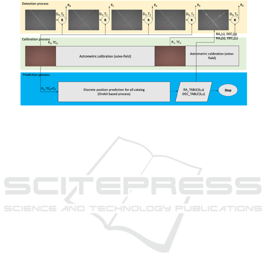
Figure 1: The solution is organized as three parallel processes: detection, calibration and prediction. Once the prediction

process finishes, the prediction data is used to interpolate the predicted satellite positions in real time.

3 SOLUTION DESCRIPTION

3.1 Batch Prediction

In order to estimate the position of the satellites

relative to the ground station observer, the following

steps are taken:

1. The latest orbital information data for known

objects is downloaded from Space-Track.org, in the

form of a list of Two-Line Elements (Kelso, 2022)

(TLEs).

2. The object detection application prepares the

prediction input, in the shape of a file containing the

GPS coordinates of the observation station, and the

time moments in the ISO 8601 format (Complete date

plus hours, minutes, seconds and decimal fraction of

a second) for which the estimations should be

performed.

3. For performing the specific orbital calculations,

the Orekit (Orekit, 2023) Java-based library is used.

For propagating the orbital TLE data, the library

implements a specific propagation class based on the

SGP4/SDP4 (Vallado, 2008) (Simplified General

Perturbation Version 4/ Simplified Deep-space

Perturbation Version 4) models. With this model,

there is a relatively low margin of error (Dong, 2010).

The propagator takes the UTC date and time

provided as input, and outputs the Position / Velocity

/ Acceleration triplet, within the ECI system (Earth

Centred, Inertial). Based on these results, and

factoring in the coordinates of the observation station,

the library can compute the topocentric equatorial

coordinates of the target, the Right Ascension and the

Declination. The 3D coordinates of the satellite are

also computed in the ECEF (Earth Centred, Earth

Fixed) reference frame, using the ITRF IERS 2010

convention. These coordinates are used for

computing the height of the satellite above the ground

surface, so that we can exclude the satellites outside

of the LEO orbit.

In order to increase the processing throughput, we

use the Java Collection API's parallelStream method,

which by default uses the Spliterator API that is

responsible for partitioning and traversing through

the given list of elements. The API's documentation

provides a clear explanation as to how it stores the

order of the elements in an encountered order, which

it will preserve in terms of the results, even if the time

it takes to process some of the data within the

different elements differs. This means that there is no

need to additionally implement a mechanism for

ordering the results. The calculations for the Position,

Velocity, Acceleration triplets for the whole time

interval are done in this fashion. By using parallel

processing, the prediction for the whole catalogue, for

two hours of look ahead time, takes less than 4

minutes on a MacBook Pro 2020 laptop.

3.2 Real Time Prediction

The result of the Orekit based prediction system is a

list of topocentric astrometric (equatorial)

coordinates, organized on two dimensions: the

discrete time intervals and the satellite numbers. The

time intervals are spaced at an interval of Q seconds

(we have experimented with Q = 60 seconds, and Q =

30 seconds. The experiments shown in this paper will

use Q = 30 seconds). The satellite number is the

ICINCO 2023 - 20th International Conference on Informatics in Control, Automation and Robotics

564

position of its orbital information in the 3le.txt file

downloaded from space-track.org, which maintains a

catalogue of more than 25000 orbital objects.

For each combination of discrete time and

satellite number, the following information is stored:

the Right Ascension and the Declination coordinates,

the 3D coordinates in the ECEF coordinate system,

the satellite name, and the satellite’s NORAD ID.

These data will be loaded into 2D arrays as soon as

the Orekit based prediction process is completed.

In order to project the astrometric coordinates into

the image space, we need to know their relation to the

image pixels. This calibration is based on

identification of the background stars, which are

catalogued and their coordinates are known. The tools

available from Astrometry.net are able to detect and

recognize the stars from any image, without prior

knowledge about the orientation of the camera or the

pixel’s angular size. The main drawback of these

tools is that they can be slower than our real time

requirement, and, at least when concerned about real

time operation, we cannot afford to calibrate each

acquired image.

The calibration will be performed in a parallel

process, for every one in 20 acquired frames. For a

time interval of 4 seconds between frames, this means

that the process will calibrate every 1:20 minutes. The

latest calibration results will be timestamped with the

time of the image used for the calibration. We’ll

denote this timestamp as T

, the time of the latest

successful calibration.

For every acquired frame that will be processed in

real time, we’ll have the current timestamp T. The

time difference between the current time and the time

of the latest successful calibration will be denoted as

∆𝑇



∆𝑇



𝑇𝑇



(1)

As the Earth rotates between observations, the

stars will change their position in the image. For a

successful association between astrometrical

coordinates and the image pixels, the time difference

between the current frame and the calibration frame

has to be taken into consideration.

For predicting the position of the satellites for the

currently acquired image, we first need to identify the

discrete time intervals in the prediction table that

encompass the current time. First, we compute the

difference between the current time T and the time of

the first prediction, T

∆𝑇



𝑇𝑇



(2)

Then, we compute the relative time ratio between the

current timestamp and the initial prediction time:

𝑘

∆𝑇



𝑄

(3)

The past and the future discrete time ratios will be

computed as:

𝑘



𝑘

(4)

𝑘



𝑘



1 (5)

The indices k

and k

are used to identify the rows in

the prediction arrays that show the position of the

satellites for the nearest past discrete time (k

) and for

the nearest future discrete time (k

). Using these two

time instances, the endpoint coordinates for the

satellite’s trajectory can be read, for each satellite s:

𝑅𝐴



𝑠  𝑅𝐴

𝑇𝐴𝐵𝐿𝐸𝑘



,𝑠 (6)

𝑅𝐴



𝑠  𝑅𝐴

𝑇𝐴𝐵𝐿𝐸𝑘



,𝑠

(7)

𝐷𝐸𝐶



𝑠  𝐷𝐸𝐶

𝑇𝐴𝐵𝐿𝐸𝑘



,𝑠

(8)

𝐷𝐸𝐶



𝑠  𝐷𝐸𝐶

𝑇𝐴𝐵𝐿𝐸𝑘



,𝑠 (9)

When the camera is fixed with respect to the ground,

the Declination coordinate corresponding to a pixel in

the image is fixed, but the Right Ascension changes

as time passes. Due to the fact that the calibration

happens at time T

, the current frame is acquired at

time T, and the endpoints of the predicted satellite

trajectories have their own timestamps (integer

multiples of Q added to the initial prediction time T

we need to correct the Right Ascension coordinates

of the two endpoints, to match their coordinates to the

pixels of the current frame:

𝑅𝐴′





𝑠



𝑅𝐴





𝑠







𝑘



𝑘



𝑄∆𝑇



𝜔

(10)

𝑅𝐴′





𝑠



𝑅𝐴





𝑠







𝑘



𝑘



𝑄∆𝑇



𝜔

(11)

𝜔

15  1.0027379043

3600

𝑑𝑒𝑔𝑟𝑒𝑒𝑠/𝑠

(12)

In equations 10, 11 and 12, 𝜔 denotes the angular

rotation speed of the Earth around its own axis, in

degrees per second. All times are expressed in

seconds, and all angles are expressed in degrees.



𝑥



,𝑦





𝑤𝑐𝑠

𝑟𝑑2𝑥𝑦𝑅𝐴′



,𝐷𝐸𝐶′



 (13)



𝑥



,𝑦





𝑤𝑐𝑠

𝑟𝑑2𝑥𝑦𝑅𝐴′



,𝐷𝐸𝐶′





(14)

In equations 13 and 14, the function wcs_rd2xy is

provided by Astrometry.net, and will map the

astrometrical coordinates to the image coordinates

based on the existing calibration parameters. The

satellite index s has been removed from the equations

for the sake of readability.

Real Time Orbital Object Recognition for Optical Space Surveillance Applications

565

Now that the endpoints of the satellite trajectory

are known, we can also approximate the position of

the satellite in the current frame. For that, we will

assume that, at least for a limited amount of time Q,

the satellite will have a linear trajectory in the image,

with constant speed. Therefore, we will use linear

interpolation for obtaining the instantaneous image

position (x, y):

𝑥𝑥





𝑘



𝑘



𝑥



𝑘  𝑘





(15)

𝑦𝑦





𝑘



𝑘



𝑦



𝑘  𝑘





(16)

The predicted trajectories and positions can now

be superimposed on the acquired image, as we can see

in Figure 2. Not all satellites in the catalogue are used

for prediction: first, based on the 3D coordinates

produced by Orekit, we exclude the satellites that

have an altitude of more than 2500 km above the

Earth surface, because they will not be visible

anyway. Then we exclude those satellites that have

the astrometric coordinates of the trajectory endpoints

too far from the astrometric coordinates of the image

centre. This way we exclude the satellites that do not

have any chance of passing through our field of view.

Figure 2: Multiple satellite predictions superimposed on the

acquired image. The line denotes the trajectory for a 30

seconds time interval, and the cross denotes the satellite’s

current predicted position. The satellite name and the

altitude above the ground are also displayed.

3.3 Detection of Satellite Streaks

The purpose of the system is Space Surveillance,

which means observation of a wider field of view,

mainly for discovering new objects or to update the

orbital parameters of some objects that have their

orbit altered periodically (newly launched objects, or

decaying objects pending re-entry in the atmosphere).

Our system relies on a Canon lens of 85 mm and

F/1.8 aperture, which ensures a field of view of 15x10

degrees. The camera is a Canon EOS 800 D DSLR

camera, acquiring images of 2400x1600 pixels. The

camera is set to operate in external trigger, pulse

width exposure control mode, so that we can precisely

timestamp the images and also control the exposure

time from the acquisition control program.

The camera is fixed with respect to the ground, an

observation setup known as “staring”. A more precise

observation strategy is the sidereal tracking approach,

where the camera is mounted on a system that

compensates the Earth’s rotation and makes the stars

appear fixed in the image. Such a mount is more

expensive, and reduces the portability of the system.

The exposure time is set at 1.5 seconds. A larger

exposure will generate longer satellite streaks, but

will also cause the stars to appear elongated due to the

Earth’s motion. The images are captured and

transferred to a host PC via the USB connection. Each

image file is assigned a timestamp from a GPS based

synchronization system.

The image processing algorithm for detecting the

satellite tracklets has the following steps:

1. Converting the images to grayscale.

2. Estimating the background using a large

median filter.

3. Performing background subtraction.

4. Computing the differences between

successive frames, with the background

removed.

5. Applying thresholding.

6. Labelling connected components.

7. Estimating elongated shapes.

8. Forming and validating tracklets.

Connected components having elongated shape

are identified as potential satellite streaks. The

presence of clouds, atmospheric turbulence, or the

faint motion of brighter stars can cause false

positives. Most of the false positives will be

eliminated by the process of tracklet formation.

The satellite candidates are connected to form

tracklets based on collinearity criteria. Only when a

minimum of three streak candidates are combined

into a tracklet the tracklet is assumed to be a valid

detection. A more detailed description of the satellite

detection process can be found in (Danescu, 2022).

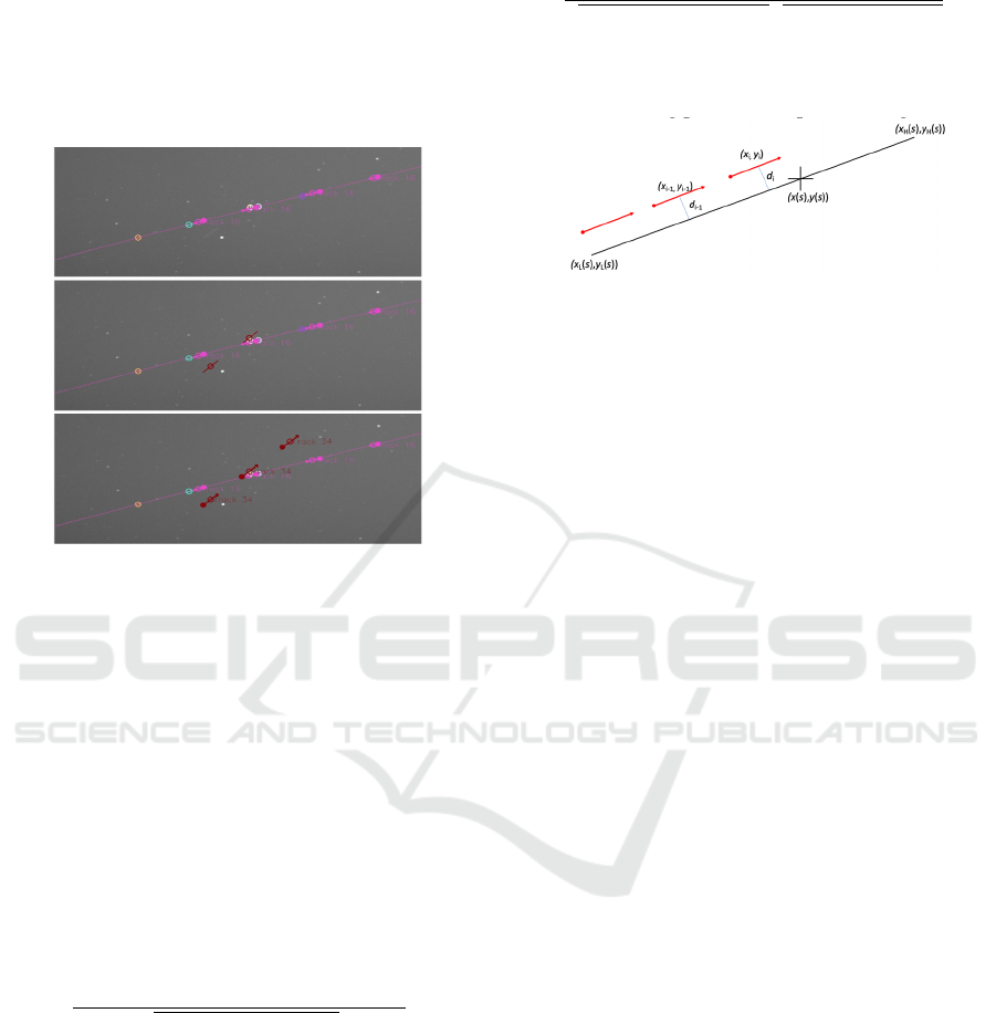
Figure 3 illustrates the tracklet formation process.

Initially, the first streak becomes visible. As the

second streak, which is collinear with the first, is

detected, the two initial results are shown as a tracklet

in phase 1 (potential but not yet valid). When three

streaks are detected, the tracklet is considered valid,

with the orientation depicted by arrows.

ICINCO 2023 - 20th International Conference on Informatics in Control, Automation and Robotics

566

Each valid tracklet contains a sequence of points

, y

), with timestamps T

. A tracklet is considered

active if it has not yet passed out of the field of view.

For example, the red tracklet of figure 3 is active,

while the pink one is not. Only the active tracklets are

considered for matching with the predicted

trajectories.

Figure 3: Detection of satellites in image sequences. Top:

initial streak becomes visible. Middle: the tracklet is

initiated, but not yet validated. Bottom: valid tracklet

showing the orientation of the motion.

3.4 Matching the Detections with the

Predicted Trajectories

For each predicted satellite s, the trajectory is defined

by the two endpoints (x

(s), y

(s)) and (x

(s), y

(s)),

and its current position is defined by the points (x(s),

y(s)). For an active track, we’ll take into consideration

the latest two detection points (middle of the streak),

, y

) and (x

i-1

, y

i-1

First, the distances between the tracklet points and

the predicted trajectory line will be computed:

𝑑







𝑥



𝑥





𝑦



𝑦









𝑥



𝑥





𝑦



𝑦







𝑥



𝑥







𝑦



𝑦







(17)

In order to accept a match between the tracklet and

the predicted trajectory, both d

and d

i-1

should be

below an acceptable threshold.

Another test is the angle between the predicted

trajectory and the tracklet trajectory. The angle

should be zero, as the two trajectories should be

parallel. The cosine of the angle between the

trajectories can be computed as:

cos 𝜑





𝑥



𝑥





𝑥



𝑥









𝑦



𝑦





𝑦



𝑦







𝑥



𝑥







𝑦



𝑦









𝑥



𝑥







𝑦



𝑦





(18)

The cos 𝜑 value should be close to 1 for parallel

trajectories. A value of 0.99 is used as a threshold.

The matching process is depicted in Figure 4.

Figure 4: Comparison between a tracklet and a predicted

trajectory.

4 TESTS AND RESULTS

4.1 Testing Setup

The testing process is performed online, during live

acquisition. The testing process has the following

steps:

1. The latest files containing updated orbital

information are downloaded from Space-

Track.org before the acquisition starts.

2. The hardware system is set up.

3. The acquisition and processing software is

started, and will produce in real time the files

containing the detection results and the

matching result.

4. The acquisition process is stopped.

5. The detection and matching results are

analysed offline for validation.

The most recent version of the system described in

this paper was tested on May 22, 2023. The

acquisition started at 22:00, and ended at 24:18.

4.2 Results

The system was able to detect a total of 231 tracklets.

Out of these tracklets, 218 were identified in real time

as belonging to known satellites, with altitudes

ranging from 400 km to 1500 km.

Not all predicted trajectories are matched with

detected tracklets, as we can clearly see from Figure

5. The matched predictions are shown as thick white

lines, while the predictions that have no tracklets

associated with them are shown with thinner white

lines and text.

Real Time Orbital Object Recognition for Optical Space Surveillance Applications

567

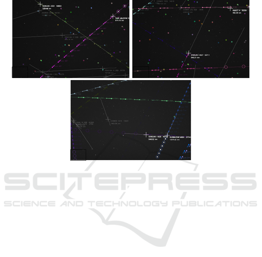
Figure 5: (a) Two satellites are detected and matched in real time, while some predicted trajectories have no associated

detections; (b) Unidentified tracklet (Track 2210, bottom of image, pink). It was later identified as a Japanese military satellite;

Of special interest are the situations when the

satellite is detected, but there is no predicted

trajectory to match it with. We had 13 such situations

for our test sequence, and they were analysed closely

offline. The offline analysis showed that:

- 8 tracklets were caused by passing planes,

which cause streaks that are similar to those

of LEO satellites;

- 2 tracklets were caused by Starlink satellites

with incorrect or outdated orbital

information;

- 3 tracklets had no explanation.

The three tracklets that still had no explanation

were tested against unofficial orbital data found at

(McCants, 2023), gathered as part of a distributed

effort to keep an eye on “classified” satellites. Based

on this data, we have identified them as military

satellites (2 belonging to the USA, and 1 belonging to

Japan). Two of them are shown in Figure 5(b) and

Figure 5(c).

5 CONCLUSIONS

In this paper we have described the solution for real

time detection and identification of satellites in the

LEO region, for wide field of view surveillance. The

solution is based on real time frame by frame

detection, and look ahead prediction of satellite

trajectories for the duration of the observation period.

The system has been tested by surveying real

satellites, in real time, and the identification

mechanism proved to work as expected.

Real time identification of surveyed satellites is

important for associating the results with the satellite

ID, for the purpose of orbital parameters refinement

and catalogue maintenance, but also for deciding

which satellites are worth a more in-depth look. A

satellite that is not matched with a predicted trajectory

can be a new, previously unknown orbital object, and

early results can lead to first estimations of its orbit.

A satellite that is on a re-entry path may also have its

orbital parameters altered, and its mismatch with the

predicted trajectory indicates that refinement of its

orbital parameters is in order.

Perhaps the most useful use of these results is in

the case of the “stare and chase” scenario. A more

accurate instrument can be oriented to better observe

a promising target, and provide more accurate results.

The integration of the real time satellite identification

within a stare and chase mechanism will be part of the

future work.

(a)

(

)

(c)

ICINCO 2023 - 20th International Conference on Informatics in Control, Automation and Robotics

568

ACKNOWLEDGEMENTS

The research was supported by a grant from the

Ministry of Research and Innovation, project number

PN-III-P2-2.1-SOL-2021-2-0192.

REFERENCES

Bland, P., Madsen, G., Bold, M., Howie, R., Hartig, B.,

Jansen-Sturgeon, T., Mason, J., McCormack, D.&

Drury, R. (2018). FireOPAL: Toward a Low-Cost,

Global, Coordinated Network of Optical Sensors for

SSA. Proceedings of the 19th AMOS (Advanced Maui

Optical and Space Surveillance Technology

Conference), USA, Sept. 5-18, 2018.

Boër, M., Klotz, A., Laugier, R., Richard, P., Dolado Perez,

J.-C., Lapasset, L., Verzeni, A., Théron, S., Coward,

D.& Kennewell, J.A. (2017). TAROT: A network for

Space Surveillance and Tracking operations.

Proceedings of 7th European Conference on Space

Debris, Darmstadt, Germany.

Ciurte, A., Soucup, A. & Danescu, R. (2014). Generic

method for real-time satellite detection using optical

acquisition systems. 2014 IEEE 10th International

Conference on Intelligent Computer Communication

and Processing (ICCP), Cluj-Napoca, Cluj, Romania,

2014, pp. 179-185.

Danescu, R., Itu, R., Turcu, V. & Moldovan, D. (2023).

Adding Surveillance Capabilities To A Leo Tracker

Using A Low-Cost Wide Field Of View Detection

System. 2nd NEO and Debris Detection Conference,

Darmstadt, Germany, 24-26 January 2023.

Danescu, R.G., Itu, R., Muresan, M.P., Rednic, A.& Turcu,

V. (2022). SST Anywhere – A Portable Solution for

Wide Field Low Earth Orbit Surveillance. Remote

Sensing, 14 (8), art no. 1905.

Diprima, F., Santoni, F., Piergentili, F., Fortunato, V.,

Abbattista, C., Amoruso, L. (2018). Efficient and

automatic image reduction framework for space debris

detection based on GPU technology. Acta Astronautica

145, 332–341.

Do, H.N.; Chin, T.J.; Moretti, N.; Jah, M.K.; Tetlow, M.

(2019). Robust foreground segmentation and image

registration for optical detection of geo objects.

Advances in Space Research, 64, 733–746.

Dong, W. and Chang-yin, Z. (2010). An accuracy analysis

of the sgp4/sdp4 model. Chinese Astronomy and

Astrophysics, 34(1):69–76.

Haimerl, J.A. & Fonder, G.P. (2015). Space Fence System

Overview. Proceedings of the 16th Advanced Maui

Optical and Space Surveillance Technology

Conference, USA, Sept. 5-18, 2015, 1-11.

Hasenohr, T. (2016). Initial Detection and Tracking of

Objects in Low Earth Orbit. Master Thesis, German

Aerospace Center Stuttgart, University of Stuttgart,

Institute of Applied Optics, 2016.

Hickson, P. (2018). A fast algorithm for the detection of

faint orbital debris tracks in optical images. Advances

in Space Research 62, 3078–3085.

Kelso, T. S. (2022). Celestrak: Norad two-line element

set format. URL https://celestrak.org/NORAD/

documentation/tle-fmt.php (Accessed May 31, 2023).

Kim, D.-W. (2016). ASTRiDE: Automated Streak

Detection for Astronomical Images. URL

https://github.com/dwkim78/ASTRiDE. (Accessed

May 24, 2023).

Lang, D., Hogg, D.W., Mierle, K., Blanton, M., Roweis, S.

(2010). Astrometry.net: Blind astrometric calibration of

arbitrary astronomical images. Astronomical Journal,

139, 1782–1800.

Langbroek, M., Bassa, C. & Molczan, T. (2023). Tracking

The Dark Side On A Shoestring Budget. 2nd NEO and

Debris Detection Conference, Darmstadt, Germany,

24-26 January 2023.

Levesque, M.P.; Buteau, S. (2007). Image Processing

Technique for Automatic Detection of Satellite Streaks.

Technical Report; Defence Research and Development:

Valcartier, QC, Canada, 2007.

LockheedMartin (2022). Space Fence. URL

https://www.lockheedmartin.com/en-us/products/spa

ce-fence.html (accessed 15 February 2022).

McCants, M. (2023). Mike McCants' Satellite Tracking

TLE ZIP Files. URL https://www.mmccants.

org/tles/index.html (accessed May 24, 2023).

Orekit (2023). Orekit - An accurate and efficient core layer

for space flight dynamics applications. URL orekit.org

(accessed May 24, 2023).

Park, J.H.; Yim, H.S.; Choi, Y.J.; Jo, J.H.; Moon, H.K.;

Park, Y.S.; Roh, D.G.; Cho, S.; Choi, E.J.; Kim, M.J.;

et al. (2018). OWL-Net: Global Network of Robotic

Telescopes for Satellites Observation. Advances in

Space Research, 62, 152–163.

SpaceTrack (2023). Space Track. URL space-track.org.

(Accessed May 24, 2023).

Vallado, D. and Crawford, P. (2008). Sgp4 orbit

determination. AIAA/AAS Astrodynamics Specialist

Conference and Exhibit, 2008.

Vananti, A., Schild, K., Schildknecht, T. (2015). Streak

Detection Algorithm For Space Debris Detection On

Optical Images. Proceedings of the 16th Advanced

Maui Optical and Space Surveillance Technology

Conference, USA, Sept. 5-18, 2015, 15–18.

Virtanen, J., Poikonen, J., Säntti, T., Komulainen, T.,

Torppa, J., Granvik, M., Muinonen, K., Pentikäinen, H.,

Martikainen, J., Näränen, J. and Lehti, J. (2016). Streak

detection and analysis pipeline for space-debris optical

images. Advances in Space Research, 57(8), pp.1607-

1623.

Wijnen, T.P.G.; Stuik, R.; Redenhuis, M.; Langbroek, M.;

Wijnja, P. (2019). Using All-Sky optical observations

for automated orbit determination and prediction for

satellites in Low Earth Orbit. Proceedings of the 1st

NEO and Debris Detection Conference, Darmstadt,

Germany, 22–24 January 2019, 1-7.

Real Time Orbital Object Recognition for Optical Space Surveillance Applications

569