Neural Network-Based Approach for Supervised

Nonlinear Feature Selection

Mamadou Kanout

e, Edith Grall-Ma

es and Pierre Beauseroy

Computer Science and Digital Society Laboratory (LIST3N), Universit

e de Technologie de Troyes, Troyes, France

Keywords:

Neural Network, Multi-Output Regression, Supervised Nonlinear Feature Selection.

Abstract:

In machine learning, the complexity of training a model increases with the size of the considered feature space.

To overcome this issue, feature or variable selection methods can be used for selecting a subset of relevant

variables. In this paper we start from an approach initially proposed for classiﬁcation problems based on a

neural network with one hidden layer in which a regularization term is incorporated for variable selection

and then show its effectiveness for regression problems. As a contribution, we propose an extension of this

approach in the multi-output regression framework. Experiments on synthetic data and real data show the

effectiveness of this approach in the supervised framework and compared to some methods of the literature.

1 INTRODUCTION

The latest technological advances allow the collection

of data from various devices . They can produce many

measurements of different types (categorical, continu-

ous) allowing them to describe the monitored system.

To infer some results not all features might be useful,

some contain no information or are redundant. To set

up a model on these data for a prediction problem, for

example, these variables must be studied to keep only

the relevant ones. Variable selection is a data analysis

technique that allows the selection of relevant vari-

ables by removing redundancy and non-informative

variables and the selection is made with respect to one

or more target variables. These target variables can be

categorical or continuous. Many methods of variable

selection have been proposed for the case of a single

target variable using statistical methods, information

theory, and neural networks and can be categorized

into three groups:

• Filter methods use statistical measures between

the target variable and other variables to select im-

portant variables such as (He et al., 2005) where

the laplacian score is used as a statistical measure.

• Wrapper methods are based on learning models

whose relevance of the selected variables depends

on the performance of the learning model, in

(Maldonado and Weber, 2009) the authors do the

feature selection using Support Vector Machine as

a learning model.

• Embedded methods add the selection constraint in

the initial formulation of the prediction model as

a regularization term to properly estimate the tar-

get variable while determining the important ones.

One of the best-known methods is Lasso (Tibshi-

rani, 2011), an approach that adds a regularization

in the formulation of a linear prediction prob-

lem to constrain weights to be sparse coefﬁcients

representing the predictor variables.

Many of these methods exploit only the linear rela-

tionships between the variables. In (Yamada et al.,

2014), (Song et al., 2012), (Song et al., 2007) the au-

thors propose a nonlinear feature selection method for

a single target variable based on Hilbert-Schmidt In-

dependence Criterion (Gretton et al., 2005), a nonlin-

ear dependency measure using kernel methods. The

complexity of this approach lies in ﬁnding the right

kernel and its parameter.

In recent years, another type of variable selection

methods in the supervised framework has attracted

the attention of researchers. It uses several target vari-

ables based on multi-task learning (Zhang and Yang,

2018), a subdomain of machine learning in which sev-

eral learning tasks are solved at the same time while

exploiting commonalities and differences between the

tasks. A good example is multi-output regression,

a regression problem with several continuous target

variables as tasks. Many applications for multi-output

regression have been studied. Approaches in the lin-

ear and nonlinear case have been proposed, in partic-

ular those using single hidden layer neural networks.

In this paper, we are interested in problems of non-

linear supervised variable selection with one or sev-

eral target variables applied to regression problems

on continuous variables. Starting from a variable se-

Kanouté, M., Grall-Maës, E. and Beauseroy, P.

Neural Network-Based Approach for Supervised Nonlinear Feature Selection.

DOI: 10.5220/0012185700003595

In Proceedings of the 15th International Joint Conference on Computational Intelligence (IJCCI 2023), pages 431-439

ISBN: 978-989-758-674-3; ISSN: 2184-3236

431

lection approach initially used for classiﬁcation prob-

lems with a single target variable, our contribution is

as follows:

• Apply this method for regression problems with a

single target variable.

• Propose an extension of this approach in the case

of selection with several target variables.

The core part of the paper is organized as follows: in

section 2, notations are introduced and related works

are detailed. In section 3, the method used as well

as its extension in the multi-output regression is ex-

posed. Experimental results are given and discussed

in section 4. Finally, in section 5 conclusions are

drawn and perspectives are proposed.

2 NOTATIONS AND RELATED

WORKS

In this section, ﬁrstly some notations used in the paper

are given and secondly an overview of previous work

related to our work is given.

2.1 Notations

The following notations are used:

• S is the set of variables in the dataset.

• S

and S

form a partition of S . They denote re-

spectively the set of target variables and the set of

predictor variables.

∪ S

= S and S

∩ S

• X and Y are matrices of observations whose vari-

ables are respectively in S

and S

• For any matrix M, the vectors M

and M

are the

row and j

column of M respectively.

• For any matrix M ∈ R

n×d

, the Frobenius norm

(Noble and Daniel, 1997) is deﬁned as follows:

||M||

tr(M

M) =

∑

1≤i≤n

∑

1≤ j≤d

i j

(1)

• For any matrix M ∈ R

n×d

, the l

2,1

norm (Ding

et al., 2006) is deﬁned as follows:

||M||

2,1

∑

i=1

∑

j=1

i j

(2)

The ||.||

2,1

norm applies the l

norm to the col-

umn elements and the l

norm to the computed

row norm. This norm, therefore, makes it possi-

ble to impose sparsity on the rows of M.

• For two matrices M ∈ R

n×d

and

M ∈ R

n×d

, the

Mean Squared Error (MSE) is deﬁned as follows:

MSE(M,

M) =

∑

j=1

∑

i=1

i j

−

i j

)

||M −

M||

(3)

2.2 Related Works

In this section, some selection methods related to our

work are described. In (Obozinski et al., 2006) the

authors propose Multi-task Lasso. It is a selection

approach based on multi-task learning, a concept al-

lowing to jointly solve several tasks deﬁned by a set

of features S

and regularization l

2,1

deﬁned in sec-

tion 2.1. Multi-task Lasso therefore makes it possible

to jointly solve several related regression tasks i.e the

variables of interest in S

by simultaneously selecting

variables in S

common to the different tasks. The

regression coefﬁcient matrix of variables noted W is

determined by minimizing the following expression:

(W ) = ||Y − XW ||

+C||W ||

2,1

, (4)

C is the regularization parameter for sparsity. The

larger is C the sparser is W . This parameter tunes

the trade-off between the estimation of the target vari-

ables and the number of selected variables. Once C

∗

the optimal C has been determined according to a cri-

terion, the importance of each variable is determined

by calculating the Euclidean norm of its correspond-

ing row in W , and variables with low impact can be re-

moved from the model. This method exploits only the

linear relationships between the variables. In (Wang

et al., 2021), the authors propose NFSN (Nonlinear

Feature Selective Networks), a nonlinear approach for

variable selection for several target variables. This

method is based on a single hidden layer neural net-

work and the addition of a regularization l

2,1

on the

weight matrix of the hidden layer for joint selection.

The expression to be optimized is:

(Θ) =

||Y −

Y ||

+C||W

(1)

2,1

(5)

where

• Θ = {W

(1)

, W

(2)

, b

(1)

, b

(2)

} is the set of neural net-

work parameters to be optimized where W

(1)

and

(2)

are respectively the weight matrices of the

hidden layer and the output layer and b

(1)

and b

(2)

are the corresponding biases.

•

Y = σ

(XW

(1)

+ b

(1)

(2)

+ b

(2)

where σ

is an

activation function.

• C is the regularization parameter for sparsity (as

deﬁned in Equation 4).

NCTA 2023 - 15th International Conference on Neural Computation Theory and Applications

432

• N is the sample size.

Once C

∗

is determined, the importance of each

variable i is determined by calculating the Euclidean

norm of its corresponding row in W

(1)

i.e ||W

(1)

These two methods allow variable selection with

several target variables, Multi-task Lasso exploits

only linear relationships between variables while

NFSN exploits nonlinear relationships between vari-

ables. In both of these approaches, the importance of

variables is determined by taking the Euclidean norm

over the rows of a weight matrix and ranking the vari-

ables according to these calculated norms. Here the

goal is to determine in a nonlinear way the coefﬁcient

associated with each variable.

3 PROPOSED APPROACH

In this part, the formulation of the based approach de-

veloped is introduced. This approach was initially in-

troduced to tackle a classiﬁcation problem. An exten-

sion of this approach is proposed for the multi-output

regression framework. In section 4 it is shown that it

can be used for regression problems.

3.1 Initial Approach for Classiﬁcation

In (Challita et al., 2016) the variable selection is

performed using a type of neural network called

Extreme learning machine (Huang et al., 2006) .

It is a neural network with one single hidden layer

where the weight matrix of the hidden layer is ran-

domly generated and not updated. Only the weight

matrix of the output layer is updated. According to

(Huang et al., 2006) these models can produce good

generalization performance and have a much faster

learning process than neural networks trained using

gradient backpropagation. The variable selection

method is based on the idea of assigning a weight to

each attribute. In the beginning, the weights of all

attributes are equal. The main goal of the method

is to adjust the weights of the different attributes to

minimize the classiﬁcation error. Attributes with

high values of weights are important and should be

kept. Attributes with low values of weights are not

important and can be removed. An illustration of the

approach is given in Figure 1.

Let N be the sample size and p the number of

variables.

Let NNeur be the number of neurons in the hidden

layer.

Let X = [a

, ··· , a

]

∈ R

p×N

where a

∈ R

is the

realisation of feature i for all observations and Y is a

vector of labels containing -1 or 1.

Figure 1: Architecture of the used approach.

The selection of features is done by minimizing

λ,C

(Θ) = ||Y −Y

+ λ||W

(2)

∑

i=1

)

(6)

where

• Y

∈ R

N×1

is the network output. It is deﬁned as

follows

= S

(2)

= σ

[(W

(1)

)

(2)

(7)

where

– σ

is an activation function. In (Challita et al.,

2016), σ

(.) = tanh(.).

– W

(1)

∈ R

NNeur×(p+1)

is the weight matrix of the

hidden layer that contains the bias coefﬁcient.

It is a random matrix.

– W

(2)

∈ R

NNeur×1

is the weight matrix of the

network output also containing the bias.

– X

= D

is a (p + 1) × N matrix whose vari-

ables are weighted

where





is (p + 1) × N matrix where 1

a vector of R

containing only 1.

∈ R

(p+1)×(p+1)

is a diagonal matrix con-

taining the weight associated with each vari-

able such that (D

)

i,i

= α

where

∈ [0, 1] is the weight associated with each

variable i for i = 1, · · · , p.

p+1

is the weight associated with the ﬁxed

input (bias). α

p+1

= 1.

• C is the regularization parameter for sparsity that

allows setting some α

to 0.

Neural Network-Based Approach for Supervised Nonlinear Feature Selection

433

• λ is the regularization parameter allowing better

stability and better generalization.

(2)

and D

are the unknowns, Θ = (W

(2)

, D

3.2 Determination of Parameters

The determination of the optimal parameters W

(2)∗

and D

∗

is crucial for estimating the target variable

and the selection of variables. To optimize the model,

(2)

and D

are updated alternately and iteratively.

That is, W

(2)

is updated with D

ﬁxed and vice versa.

is initialized as an identity matrix.

For ﬁxed D

, in (Challita et al., 2016) W

(2)

is up-

dated by calculating the derivative of Equation 6 with

respect to W

(2)

, which leads to the simple closed form

solution:

(2)∗

+ λI)

(8)

For ﬁxed W

(2)

, D

the diagonal matrix with α

its diagonal entries is updated. To take into account

the constraints on α

for i = 1, . . . , p deﬁned in sec-

tion 3.1 , the optimization problem is reformulated as

follows:

minimize

λ,C

(Θ)

subject to α

− 1 ≤ 0, −α

≤ 0, i = 1, . . . , p.

(9)

As in (Challita et al., 2016), the partial deriva-

tive of Equation 6 with respect to α

is approximated

by numerical methods. The optimization problem of

Equation 9 is solved by optimization algorithms.

3.3 Multi-Output Regression

Based on the formulation given in (Challita et al.,

2016) which is adapted to the single task problem,

a new method named FS-ELM meaning Feature Se-

lection using Extreme Learning Machine is proposed.

This method can tackle multi output regression prob-

lems where the number of variables in S

is greater

than 1. The proposed method replaces the l

norm in

the objective function and the constraint on W

(2)

the Frobenius norm where W

(2)

∈ R

NNeur×card(S

)

λ,C

(Θ) is reformulated as follows:

λ,C

(Θ) = ||Y −Y

+ λ||W

(2)

∑

i=1

)

(10)

where

• The derivative of L(Θ) with respect to W

(2)

re-

mains the same as in Equation 8.

• The update of D

remains the same as deﬁned in

Equation 9.

4 EXPERIMENTS

In this part, two sets of variables S

and S

corre-

sponding respectively to available variables and vari-

ables to be inferred are assumed to be deﬁned. The ef-

fectiveness of the proposed approach to select a subset

of relevant variables in S

for estimating S

is shown.

The subsection 4.1 is about the evaluation of FS-

ELM on synthetic data and the subsection 4.2 on real-

world data. For a single target variable, the proposed

method is compared with Lasso, NFSN, and for sev-

eral target variables, the comparison is made with

Multi-task Lasso, NFSN. To show the effectiveness

of the proposed method and to compare it with other

methods, the procedure is composed of three steps:

• Determine C

∗

and λ

∗

the optimal values of C and

λ according to a criterion on the MSE.

– for C ∈ I

with I

= {10

−4

, 10

−3

, . . . , 10

, 10

}

for λ ∈ I

with I

= {10

−4

, 10

−3

, . . . , 10

, 10

}

· Compute

(λ,C)

the estimate of Y associated

with C and λ on a train data set.

– Choose (C

∗

, λ

∗

) ∈ I

× I

such that

∗

, λ

∗

) = argmin

(C,λ)∈I

×I

MSE(Y, Y

(λ,C)

) (11)

∗

, λ

∗

) ∈ I

× I

is a pair of values that

minimize MSE(Y, Y

(λ,C)

) ∀ (C, λ) ∈ I

× I

using a test data set.

For Multi-task Lasso, NFSN and Lasso ap-

proaches where C is the only parameter to be

tuned, the procedure is similar to the one above

but only C

∗

is determined.

• Once hyperparameters are chosen, for each ap-

proach, rank the variables according to their im-

portance.

– For Lasso, rank the variables according to the

ordered values of the absolute value of the co-

efﬁcients of the linear regression model.

– For Multi-task Lasso and NFSN, rank the vari-

ables as deﬁned in section 2.2.

– For FS-ELM, rank the variables according to

the scaling factors α

• Evaluate the pertinence of ranking for each ap-

proach by building p models on the train data set

and evaluating them on the test data set by keeping

from 1 to p variables corresponding to the highest

rank.

The evaluation model used is a single hidden

layer neural network with 500 neurons. The

activation function is relu and the optimizer is

NCTA 2023 - 15th International Conference on Neural Computation Theory and Applications

434

adam.

The relevance of the selected variables is evalu-

ated using the MSE of the estimated model.

To avoid scaling problems, the variables of matrices

X and Y are normalized (a pre-processing technique

of removing the mean and scaling to unit variance ap-

plied to each variable).

The validation of the results is done by 5-fold cross-

validation.

4.1 Synthetic Data Set

Firstly, 8 Gaussian features were deﬁned. Then 10

random features that depend on these 8 Gaussian fea-

tures with nonlinear relationships were deﬁned. Fi-

nally, 4 other independent Gaussian features were

added. Then data were generated from these 22 fea-

tures as described below.

• f

∼ N (1, 5

) ; f

∼ N (0, 2

) ; f

∼ N (2, 7

)

• f

∼ N (5, 3

), f

∼ N (0, 1); f

∼ N (0, 0.3

)

• f

∼ N (3, 2

); f

∼ N (11, 1)

• f

= sin( f

) + ε

, ε

∼ N (0, 0.08

)

• f

= log(| f

|) + ε

, ε

∼ N (0, 0.08

)

• f

= cos( f

) + ε

, ε

∼ N (0, 0.1

)

• f

= f

sin(

) + ε

, ε

∼ N (0, 0.04

)

• f

= f

+ f

− f

+ f

+ ε

, ε

∼

N (0, 0.02

)

• f

= f

( f

+ log(f

)) + ε

, ε

∼ N (0, 0.08

)

• f

= f

+ f

(sin( f

+ f

)) + ε

, ε

∼

N (0, 0.08

)

• f

+ f

+ ε

, ε

∼ N (0, 0.04

)

• f

= sin(e

− f

) + ε

, ε

∼ N (0, 0.01

)

• f

= cos(sin( f

)) + ε

, ε

∼ N (0, 0.08

)

• f

, f

∼ N (0, 1).

The set of variables is S = { f

, ··· , f

}

On the generated data, experiments have been

done in two cases for S

, with S

= S \ S

For the ﬁrst experiment, S

= { f

}. Figure 2a

shows the estimated value of the mean of the MSE

for the variables of S

versus log(C). For Lasso

∗

= 10

−2

, for FS-ELM C

∗

= 10

, λ

∗

= 10

−3

and

for NFSN C

∗

= 10

−4

. After the choice of the regu-

larization parameters, the list of ranked variables for

Table 1: List of ranked variables for each approach. Vari-

ables in bold are the ideal variables that should be selected

by the approaches.

(a) S

= { f

Lasso FS-ELM NFSN

(b) S

= { f

, f

Multi-task Lasso FS-ELM NFSN

Lasso, FS-ELM and NFSN is given in Table 1. Fig-

ure 3a shows the estimated value of the mean of MSE

versus the number of most important variables used to

build the model. It may be noticed that for NFSN and

FS-ELM the ﬁrst 2 most important variables allow to

estimate well the target variable while for Multi-task

Lasso it takes the ﬁrst 14 most important variables.

As the same variables were selected by NFSN and

FS-ELM, the green curve is exactly underneath the

red curve.

For the second experiment, S

= { f

, f

Figure 2b shows the estimated value of the mean

of the MSE for the variables of S

versus log(C).

For Multi-task Lasso C

∗

= 10

−2

, for FS-ELM C

∗

, λ

∗

= 10

−1

, for NFSN C

∗

= 10

−3

. Table 1b con-

tains the list of ranked variables for Multi-task Lasso,

FS-ELM and NFSN after the choice of regulariza-

tion parameters. Figure 3b shows the estimated value

of the mean of MSE versus the number of most im-

portant variables taken. It may be noticed that for

NFSN and FS-ELM the ﬁrst 3 most important vari-

ables allow to estimate well the target variable while

for Lasso it takes the ﬁrst 6 most important variables.

4.2 Real-World Data Sets

In this part, the proposed method is evaluated on the

real-world data sets and compared to other methods

for one and several target variables. Table 2 contains

the list of real-world data used as well as the number

of target variables, number of predictor variables, and

number of samples. Some information about the data

sets in Table 2 as well as the pre-processing of data

Neural Network-Based Approach for Supervised Nonlinear Feature Selection

435

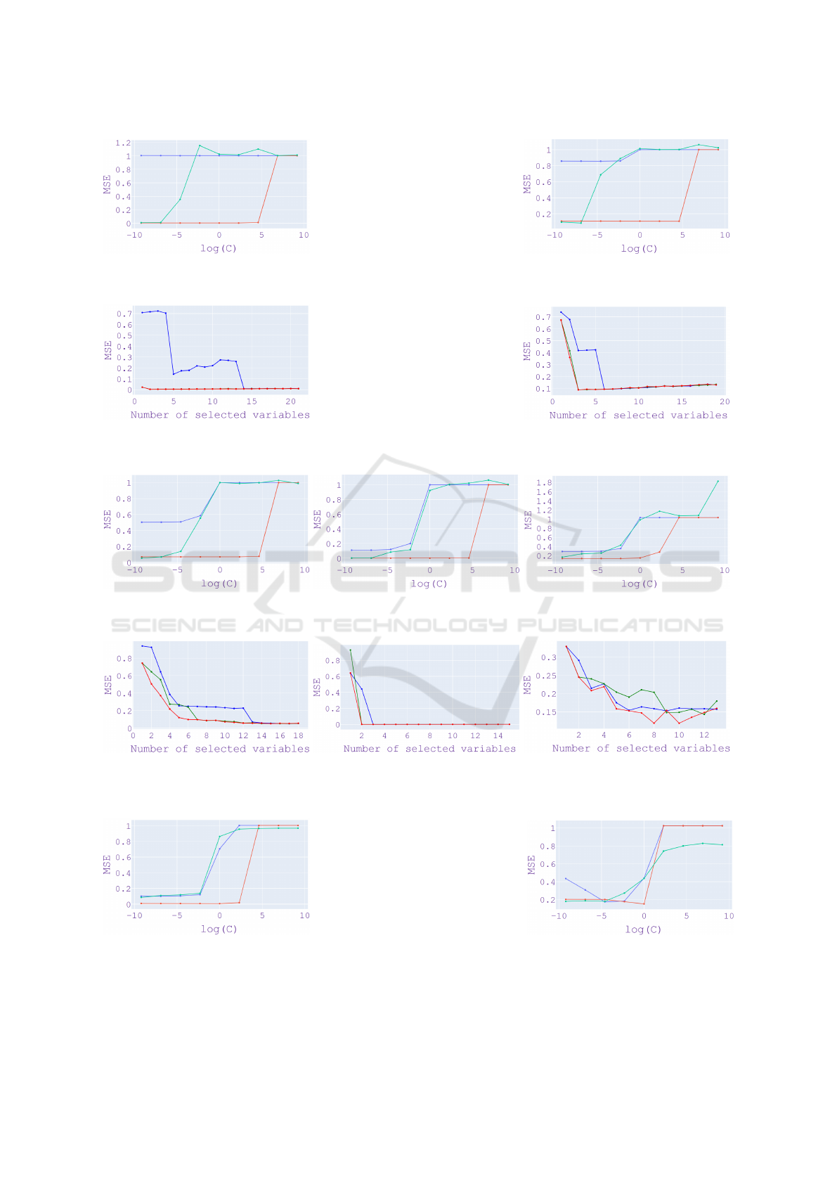
(a) S

= { f

} and S

= S \ S

. (b) S

= { f

, f

} and S

= S \ S

Figure 2: MSE versus log(C) on synthetic data. Lasso (blue), NFSN (green), FS-ELM (red).

(a) S

= { f

} and S

= S \ S

. (b) S

= { f

, f

} and S

= S \ S

Figure 3: MSE versus number of most important variables on synthetic data. Lasso (blue), NFSN (green), FS-ELM (red).

(a) Bike sharing data set. (b) Air quality data set. (c) Boston house data set.

Figure 4: MSE versus log(C) on real-world data with a single target. Lasso (blue), NFSN (green), FS-ELM (red).

(a) Bike sharing dataset. (b) Air quality data set. (c) Boston house data set.

Figure 5: MSE versus number of important variables to keep for selection with a single target variable on real-world data sets.

Lasso (blue), NFSN (green), FS-ELM (red).

(a) Enb data set. (b) Atp1d data set.

Figure 6: MSE versus log(C) on real-world data sets with several target variables. Multi-task Lasso (blue), NFSN (green),

FS-ELM (red).

NCTA 2023 - 15th International Conference on Neural Computation Theory and Applications

436

(a) Enb data set. (b) Atp1d data set.

Figure 7: MSE versus the number of most important variables on real-world data sets with several target variables. Multi-task

Lasso (blue), NFSN (green), FS-ELM (red).

done are described below.

• Bike sharing dataset

This data set contains monitoring data of rental

bike users in a city with 16 variables including one

target variable and 15 predictor variables. Only

the ﬁle ”hour.csv” on UCI website is used in this

paper. Among the 15 predictors variables, 7 vari-

ables are continuous, 3 variables are binary cate-

gorical and 5 are cyclical discrete variables. The

sine and cosine transformation is applied to the

cyclic variables, they are then removed and the

continuous variables are normalized. The selec-

tion approaches are applied to the obtained 20

variables in order to estimate the target variable.

• Air quality dataset

This data contains the responses of a gas multi-

sensor device deployed on the ﬁeld in an Italian

city. It is composed of 15 variables including a

target variable and 14 predictors variables includ-

ing 12 continuous variables, a time variable and

a date variable. A new variable called month is

deduced from the variable date and the variable

called hour is deduced from variable time. The

sine and cosine transformation is applied to the

cyclic variables month and hour, they are then re-

moved. The selection approaches are applied to

17 variables for estimating the target variable.

• Boston house

This data set contains information collected by

the U.S Census Service concerning housing in the

area of Boston Mass. There are 14 variables in-

cluding one target variable and 13 continuous pre-

dictor variables.

• Enb dataset

This data set of 10 variables includes 2 target vari-

ables the heating load and cooling load require-

ments of the building and 8 continuous predictor

variables such as glazing area, roof area, and over-

all height, . . . The data set is taken from Mulan, an

open-source Java library for learning from multi-

label data sets and it can also be downloaded from

Table 2: Real-world data sets for variable selection.

Name Size Features Targets Source

Bike sharing 17 389 15 1 (Fanaee-T and Gama, 2013)

Air quality 9 357 14 1 (De Vito et al., 2008)

Boston house 506 13 1 (Harrison and Rubinfeld, 1978)

Enb 768 8 2 (Tsanas and Xifara, 2012)

Atp1d 337 411 6 (Xiouﬁs et al., 2012)

their github https://github.com/tsoumakas/mulan.

• Atp1d

This dataset of 337 observations is about the pre-

diction of airline ticket prices. There are 417 vari-

ables including 6 variables as targets and 411 pre-

dictor variables. The data set is taken from Mulan.

The cases with one target are ﬁrst tackled. Fig-

ure 4 shows the estimated value of the mean of the

MSE between Y and its estimate versus log(C) by 5-

fold cross-validation for each approach on the Bike

sharing, Air quality, and Boston data sets. It can be

noticed the stability of performance of FS-ELM for

large values of C compared to other methods.

For each approach and each data set, the chosen C

∗

described below:

• On Bike sharing dataset, C

∗

= 10

−4

for Lasso,

∗

= 10, λ

∗

= 10

−4

for FS-ELM and C

∗

= 10

−4

for NFSN.

• On Air quality dataset, C

∗

= 10

−4

for Lasso, C

∗

−1

, λ

∗

= 10

−1

for FS-ELM and C

∗

= 10

−4

for

NFSN.

• On Boston house dataset, C

∗

= 10

−4

for Lasso,

∗

= 10

−1

, λ

∗

= 10

−2

for FS-ELM and C

∗

= 10

−4

for NFSN.

Once the regularization parameters have been de-

termined for each approach, the most important vari-

ables are taken gradually, then an estimate is made

to assess the relevance of the variables taken and

to determine the number of variables to keep. The

number of important variables taken successively is

{1, 2, . . . , 20} on Bike sharing data set, {1, 2, . . . , 17}

on Air quality data set and {1, 2, . . . , 13} on Boston

house data set. Figure 5 shows the MSE between Y

and its estimate versus the number of important vari-

ables taken successively for each approach on Bike

Neural Network-Based Approach for Supervised Nonlinear Feature Selection

437

sharing, Air quality, Boston house data sets. It can

be noticed that in general FS-ELM manages to select

the variables better compared to the other approaches.

Precisely:

• On Bike sharing data set, FS-ELM performs well

in the variable selection compared to Lasso and

NFSN.

• On Air quality data set, the two ﬁrst important

variables selected by FS-ELM and NFSN can es-

timate well the target variable.

• On the Boston house data set, FS-ELM performs

well compared to NFSN. Indeed, FS-ELM has the

minimum MSE for any number of selected vari-

ables. There are some variances in the MSE be-

cause there are only 508 samples.

Figure 6 shows the estimated value of the mean of

the MSE by 5-fold cross-validation between Y and its

estimate versus log(C) for each approach on the data

sets with several target variables. It can be noticed

that FS-ELM has greater stability for regularization

parameters than the other methods. For each approach

and each data set, the chosen C

∗

is described below:

• On Enb data set, C

∗

= 10

−4

for Multi-task Lasso,

∗

= 1, λ

∗

= 10

−3

for FS-ELM, C

∗

= 10

−4

for

NFSN.

• On Atp1d data set, C

∗

= 10

−2

for Multi-task

Lasso, C

∗

= 1, λ

∗

= 10

−2

for FS-ELM, C

∗

= 10

−2

for NFSN.

Once the regularization parameters have been

determined for each approach, the variables are

ranked for each approach. The number of important

variables taken successively is {1, 2, . . . , 8} on Enb

data set and {50, 100, 150, . . . , 400} on Atp1d data

set. Figure 7 shows the estimated value of the mean

of the MSE by 5-fold cross-validation between Y and

its estimate versus the number of important variables

taken successively for each approach and on the data

sets Enb, Atp1d. It can be noticed that in general,

FS-ELM manages to select well the relevant variables

and reach the best performance with Atp1d which is

the most challenging case.

The proposed method successfully selects the rel-

evant variables on regression problems for one and

several target variables. In addition, it can be no-

ticed that generally, FS-ELM selects better compared

to NFSN and Multi-task Lasso.

5 CONCLUSIONS

In this paper, starting from an approach that was ini-

tially proposed for a classiﬁcation problem with a

single target variable, we ﬁrst showed its feasibility

for regression problems with a single target variable,

then proposed an extension in the framework of multi-

output regression for variable selection with several

target variables. Finally, many experiments made on

synthetic data and real data conﬁrm the effectiveness

of the proposed approach.

The future works would be to:

• Calculate the partial derivative of L

λ,C

(Θ) with re-

spect to the α

since it was not calculated in the

initial formulation and this work to improve the

optimization algorithm.

• Propose an approximation of the matrix division

made in Equation 8 to reduce the complexity of

the optimization.

• Apply the proposed extension to the unsupervised

nonlinear variable selection problems for contin-

uous variables.

ACKNOWLEDGEMENT

This work was supported by Labcom-DiTeX, a joint

research group in Textile Data Innovation between In-

stitut Franc¸ais du Textile et de l’Habillement (IFTH)

and Universit

e de Technologie de Troyes (UTT).

REFERENCES

Challita, N., Khalil, M., and Beauseroy, P. (2016). New

feature selection method based on neural network and

machine learning.

De Vito, S., Massera, E., Piga, M., Martinotto, L., and

Francia, G. (2008). On ﬁeld calibration of an elec-

tronic nose for benzene estimation in an urban pol-

lution monitoring scenario. Sensors and Actuators B

Chemical.

Ding, C., Zhou, D., He, X., and Zha, H. (2006). R 1-

pca: Rotational invariant l 1-norm principal compo-

nent analysis for robust subspace factorization. In

ICML 2006 - Proceedings of the 23rd International

Conference on Machine Learning.

Fanaee-T, H. and Gama, J. (2013). Event labeling combin-

ing ensemble detectors and background knowledge.

Progress in Artiﬁcial Intelligence.

Gretton, A., Bousquet, O., Smola, A., and Sch

olkopf, B.

(2005). Measuring statistical dependence with hilbert-

schmidt norms.

Harrison, D. and Rubinfeld, D. (1978). Hedonic housing

prices and the demand for clean air. Journal of Envi-

ronmental Economics and Management.

He, X., Cai, D., and Niyogi, P. (2005). Laplacian score for

feature selection.

NCTA 2023 - 15th International Conference on Neural Computation Theory and Applications

438

Huang, G., Zhu, Q.-Y., and Siew, C. K. (2006). Extreme

learning machine: Theory and applications. Neuro-

computing.

Maldonado, S. and Weber, R. (2009). Weber, r.: A wrap-

per method for feature selection using support vector

machines. inf. sci. 179(13), 2208-2217.

Noble, B. and Daniel, J. W. (1997). Applied linear algebra.

2nd ed.

Obozinski, G., Taskar, B., and Jordan, M. (2006). Multi-

task feature selection.

Song, L., Bedo, J., Borgwardt, K. M., Gretton, A., and

Smola, A. (2007). Gene selection via the bahsic fam-

ily of algorithms. volume 23, pages i490–i498. Bioin-

formatics.

Song, L., Smola, A., Gretton, A., Bedo, J., and Borgwardt,

K. (2012). Feature selection via dependence maxi-

mization. JMLR.org.

Tibshirani, R. (2011). Regression shrinkage selection via

the lasso. In Journal of the Royal Statistical Society

Series B.

Tsanas, A. and Xifara, A. (2012). Accurate quantitative

estimation of energy performance of residential build-

ings using statistical machine learning tools. Energy

and Buildings.

Wang, Z., Nie, F., Zhang, C., Wang, R., and Li, X. (2021).

Joint nonlinear feature selection and continuous val-

ues regression network.

Xiouﬁs, E. S., Groves, W., Tsoumakas, G., and Vlahavas,

I. P. (2012). Multi-label classiﬁcation methods for

multi-target regression. CoRR.

Yamada, M., Jitkrittum, W., Sigal, L., Xing, E. P., and

Sugiyama, M. (2014). High-dimensional feature se-

lection by feature-wise kernelized lasso. MIT Press -

publishers.

Zhang, Y. and Yang, Q. (2018). An overview of multi-task

learning.

Neural Network-Based Approach for Supervised Nonlinear Feature Selection

439