Testing Variants of LSTM Networks for a

Production Forecasting Problem

Nouf Alkaabi

, Sid Shakya

and Rabeb Mizouni

Electrical and Computer Engineering Dept., Khalifa University, Abu Dhabi, U.A.E.

EBTIC, Khalifa University, Abu Dhabi, U.A.E.

Computer Engineering Dept., Khalifa University, Abu Dhabi, U.A.E.

Keywords:

Time Series Analysis, LSTM, Forecasting, Sequential Features, Non-Sequential Features.

Abstract:

Forecasting the production of essential items such as food is one of the issues that many retail authorities

encounter frequently. A well-planned supply chain will prevent an under- and an oversupply. By forecasting

behaviors and trends using historical data and other accessible parameters, AI-driven demand forecasting

techniques can address this problem. Earlier work has focused on the traditional Machine Learning (ML)

models, such as Auto-Regression (AR), Auto-regressive Integrated Moving Average (ARIMA), and Long

Short-Term Memory (LSTM) for forecasting production. A thorough experimental analysis demonstrates that

various models can perform better in various datasets. However, with additional hyper-parameters that may

be further tweaked to increase accuracy, the LSTM technique is typically the most adaptable. In this work,

we explore the possibility of incorporating additional non-sequential features with the view of increasing the

accuracy of the forecast. For this, the month of production, temperature, and the number of rainy days are

considered as additional static non-sequential features. There are various ways such static features can be

incorporated in a sequential model such as LSTM. In this work, two variants are built, and their performances

for the problem of food production forecasting are compared.

1 INTRODUCTION

Forecasting the production of essential items such

as food is a crucial problem that decision-makers at

many private and public authorities ﬁnd challenging.

The ability to accurately estimate expected produc-

tion is crucial for supply chain planning, which avoids

waste by regulating expected production against ex-

pected import.

time series forecasting techniques are being used for

demand forecasting to predict behaviors and trends

reliably. Particularly, regression techniques such as

AR (Ullrich, 2021) and ARIMA (Shumway and Stof-

fer, 2017) are the simplest techniques and usually the

fastest to execute. However, they might result in low

prediction accuracy. Machine Learning (ML) and

Deep Learning (DL) techniques, on the other hand,

can perform better but may require higher computa-

tion time and also require a proper setup of hyperpa-

rameters to ﬁne-tune models. One of the famous DL

techniques used to represent sequential data is the Re-

current Neural Networks (RNNs) (Salehinejad et al.,

2017). RNNs are Artiﬁcial Neural Networks (ANNs)

(Burden and Winkler, 2009) with recurrent connec-

tions made up of nonlinear hidden states with high

dimensions. The network’s memory comprises hid-

den state structures, and each hidden layer’s current

state depends on its previous state. The three layers

of RNN are the input, recurrent hidden, and output.

Nonlinear state equations that can be repeatedly iter-

ated make up the RNN. The hidden states provide an

output layer prediction depending on the input vec-

tor at each timestep. A set of values known as an

RNN’s hidden state contains all the necessary infor-

mation about the network’s earlier states over many

timesteps, irrespective of any outside inﬂuences. The

network’s future behavior can be predicted using the

combined data, which allows the output layer to make

precise predictions.

A unique variant of RNNs called LSTM (Hochre-

iter and Schmidhuber, 1997) can learn long-term de-

pendencies and deal with the vanishing gradient prob-

lem (Van Houdt et al., 2020) that RNNs suffer from

and is considered a powerful tool in dealing with

complex time series forecasting problems. A typical

LSTM has three gates: a forget gate, an input gate,

524

Alkaabi, N., Shakya, S. and Mizouni, R.

Testing Variants of LSTM Networks for a Production Forecasting Problem.

DOI: 10.5220/0012186100003595

In Proceedings of the 15th International Joint Conference on Computational Intelligence (IJCCI 2023), pages 524-531

ISBN: 978-989-758-674-3; ISSN: 2184-3236

and an output gate. These gates can be thought of as

ﬁlters. More details about RNN and LSTM can be

found in (Salehinejad et al., 2017) and (Van Houdt

et al., 2020).

In this paper, we study real-world data from

our partner organization and investigate the effect of

adding non-sequential features to the model. The ob-

jective is to increase the forecast accuracy. For this,

we use three static features, the production month,

the temperature, and the number of rainy days, as

additional static features and study different ways to

incorporate them in a sequential LSTM framework.

Notably, the production month was derived from the

DateTime information in the dataset. In fact, food

production has a seasonal effect and is inﬂuenced by

the month of its production, and thus, we have in-

corporated it as a parameter to emphasize its impor-

tance. Additionally, we augmented the dataset by

integrating other static features, temperature and the

number of rainy days, from different sources to cap-

ture the inﬂuence of weather conditions on productiv-

ity. By considering these factors, we expect to gain

a deeper understanding of the complex interplay be-

tween weather and food production, resulting in more

accurate forecast.

We investigate two ways of incorporating those static

features into the sequential model.

1. By replicating the static feature in the sequence as

a ﬁxed temporal parameter

2. By designing a multi-headed network with an ad-

ditional feed-forward layer to consider the ﬁxed

parameter input.

The rest of the paper is organized as follows. Sec-

tion 2 presents the background of the applied LSTM

model and reviews some of the previous work done in

this area. Section 3 presents the methodology, where

two proposed approach of incorporating static fea-

tures in the sequential model is described. Section

4 describes experimental setups and presents the re-

sults. Finally, section 5 summarizes the paper and

highlights future work.

2 BACKGROUND

Time series are generally affected by four essential

components: trend, seasonal, cyclical, and irregular

components. When a time series exhibits an upward

or downward movement in the long run, it can be

asserted that the series has a general trend. Gener-

ally, the trend is a Long-term increase or decrease

in the data over time. When a series is affected by

seasonal factors, a seasonality pattern exists, such as

quarterly, yearly, monthly, weekly, and daily patterns.

The cyclic occurs when data rises and falls, which

means it is not a ﬁxed period. The cycle duration is

over a long period, which may be two years or more.

The irregular component, sometimes known as the

residual, refers to the variation that exists because of

unpredictable factors. More details about the time se-

ries and its components can be found in (Jose, 2022).

Many different ML techniques are used to solve dif-

ferent time series forecasting problems. The authors

of (Mahmud and Mohammed, 2021) conduct a survey

that studies and compares the efﬁcacy of time series

models to make predictions of real data. According

to the authors, LSTMs have proven to perform well

and are relatively easy to train. Therefore, LSTMs

have become the baseline architecture for tasks where

it is necessary to process sequential data with tempo-

ral information. An application of forecasting ﬁnan-

cial data was reported with two tested models, LSTM

and ARIMA, where the results show that LSTM was

a better predictor than ARIMA. LSTM was the best

approach for another reported application by Fischer

and Krauss (Fischer and Krauss, 2018) for stock pre-

diction. LSTM was compared to memory-free algo-

rithms such as Random Forest (Liu et al., 2012), Lo-

gistic Regression Classiﬁer (Peng et al., 2002), and

Deep Neural Network (Burden and Winkler, 2009).

Some approaches have also been proposed in litera-

ture targeting food production forecasting. One ex-

ample can be found in (Kamran et al., 2019), where

the authors predict Wheat Production in Pakistan us-

ing LSTM. Their proposed mechanism was compared

with a few existing models in the literature, such as

ARIMA and RNN. They concluded that the proposed

LSTM model achieves better performance in terms

of forecasting. Another approach was proposed in

(Livieris et al., 2020) for predicting the future prices

of gold using a combination of Convolutional Neu-

ral Networks (CNN) and LSTM networks. The CNN

component of the model is responsible for extract-

ing relevant features from the input data, while The

LSTM component takes the sequential nature of the

time series into account and captures long-term de-

pendencies by learning from past data. The experi-

mental results show that the CNN-LSTM model out-

performs the other models in terms of forecasting ac-

curacy. It demonstrates the ability to capture both lo-

cal and global patterns in the gold price time series,

leading to more accurate predictions. Moreover, a

novel approach was proposed in (Sagheer and Kotb,

2019), where a method for predicting petroleum pro-

duction using deep LSTM (DLSTM) was presented.

The proposed architecture could capture the complex

patterns and dynamics present in petroleum produc-

Testing Variants of LSTM Networks for a Production Forecasting Problem

525

tion time series data. A genetic algorithm was applied

in order to optimally conﬁgure DLSTM’s optimum

architecture. Experimental results demonstrate that

the deep LSTM network achieves superior forecast-

ing accuracy compared to traditional methods such

as ARIMA and single-layer LSTM networks. In

(Alkaabi and Shakya, 2022), an LSTM was tested

against classical machine learning time series analy-

sis models, such as AR (Ullrich, 2021) and ARIMA

(Shumway and Stoffer, 2017), for production fore-

casting, which conclude that the LSTM approach is

generally the most ﬂexible approach, with more hy-

perparameters that can be further tuned to improve

accuracy.

3 METHODOLOGY

We investigate the effect of static non-sequential fea-

tures together with sequential production data, with

the view of improving the overall accuracy. By con-

sidering these static variables alongside the sequen-

tial data, we anticipate discovering novel patterns and

relationships that might have been overlooked pre-

viously. By incorporating static non-sequential fea-

tures, we introduce a new dimension to the model’s

analysis. This addition allows us to capture contex-

tual information that can potentially enhance the ac-

curacy and effectiveness of the sequential model. We

believe that by examining the interplay between the

static and sequential features, we can gain deeper in-

sights into the underlying dynamics of the system un-

der investigation. However, static data cannot be nat-

urally added to the LSTM model due to it being a

sequential model; hence we investigate two different

ways to achieve this.

A multiyear time series dataset was used. This

dataset consists of a single column representing the

monthly production values of various food items. The

dataset was enriched by combining it with another

dataset that contains the monthly temperature and

rainy days to create a multivariate dataset. We sep-

arate the data into training and testing sets, with the

testing set being the dataset’s most recent 12 months

of production. For the purpose of this paper, we

choose six sample products (referenced as p1, p2,

..,p6 for anonymity), representing typical products in

the full dataset, consisting of different distributions.

We device four different topologies of LSTM with

the above dataset and compare their performance.

The ﬁrst model, M1, consists of a simple univariate

LSTM model that only includes the sequential histor-

ical production data but excludes the additional non-

sequential data, such as the month of production and

the temperatures. The second model, M2, consists of

a multivariate LSTM model where the static values

were replicated for each time series period to emulate

the sequential representation required by LSTM. The

third and fourth models, M3 and M4, respectively,

consist of two different conﬁgurations of a multi-

headed approach where an LSTM was combined with

a traditional Feed-Forward Neural Network (FFN).

Here, LSTM was used for sequential production data,

and the FFN was used for static data. In particular,

the outputs of LSTM cells were combined with static

input data and passed to FFN to produce the ﬁnal pre-

diction.

The models’ parameters were tuned empirically,

where we performed multiple experiments with many

settings for the hyperparameters and chose the set-

tings that resulted in the best accuracy. However,

some hyperparameters were set to be the same for all

models as to provide a fair comparison, such as the

sequence size for LSTM (aka lag parameter), the op-

timizer, and the number of epochs. The lag param-

eter was set to 12 to use the past 12 months to pre-

dict 13

month, the optimizer was set to Adam op-

timizer (Kingma and Ba, 2014), and the number of

epochs was set to 100, with early stopping criteria im-

plemented to prevent overﬁtting.

3.1 M1: Univariate LSTM

The ﬁrst model tested was a univariate LSTM model.

The model consists of a single LSTM layer, with eight

units, that takes as an input a sequence of 12 months’

production values and predicts the 13

month. The

input of the LSTM is represented in Figure 4. The

output of the LSTM layer is then passed to a Dense

layer with one neuron to produce one ﬁnal output.

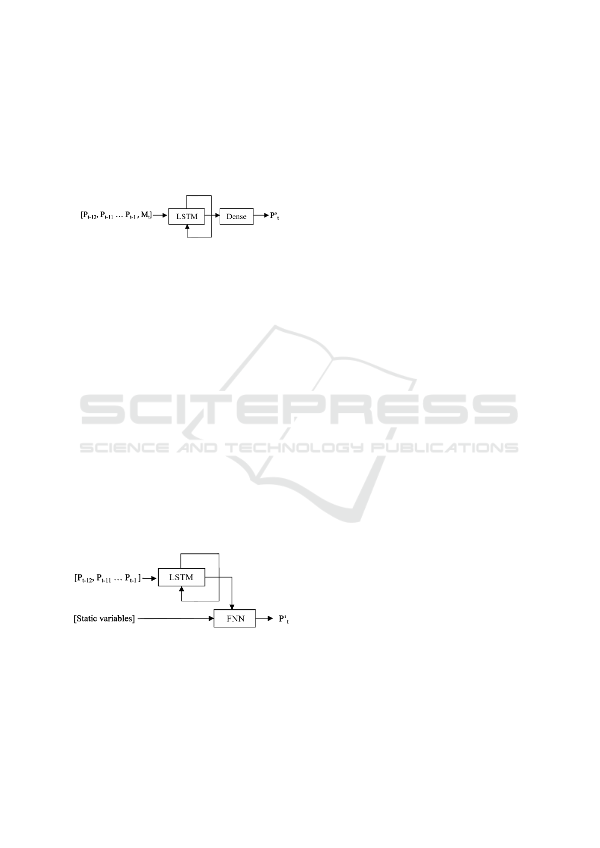
Figure 1 represents the model at the timestep where

the production P at time t will be predicted.

Figure 1: M1: Univariate LSTM model.

3.2 M2: Multivariate LSTM

The topology of M2 is similar to the topology of

M1, except that it has an additional parameter that

represents the prediction month. Since the predic-

tion month is ﬁxed, this parameter has to be repli-

cated 12 times for each timestep in order to produce

a ﬁxed temporal parameter. Hence, each input sam-

ple received by the LSTM layer consisted of two fea-

NCTA 2023 - 15th International Conference on Neural Computation Theory and Applications

526

tures. The ﬁrst is the production value at the time t −i,

where i = [1,2, ..., 12], along with a constant param-

eter M

representing the month to be predicted. Also,

the month’s value is preprocessed using a one-hot en-

coding before passing it to the LSTM layer. The in-

put of the model is represented in Figure 5. Figure 2

shows the model when the production P at time t is to

be predicted.

Figure 2: M2: Multivariate LSTM model.

3.3 M3 and M4: Multi-Headed LSTM

Models

These two models combine LSTM with FNN to create

a multi-headed model. Instead of repeatedly passing

the value of the predicted month to the LSTM net-

work, we add the predicted month as an additional

categorical static feature to the output of a univari-

ate LSTM layer that takes a sequence of the past 12

months. The combination of those two is passed to

FNN with two Dense layers. Here, FNN also acts as

the ﬁnal layer. Similar to M2, the predicted month

here is one-hot encoded. Figure 6 shows the input of

M3.

M4 further extends this approach and investigates the

effect of two more static features on the overall accu-

racy, namely, the temperature and the number of rainy

days of the predicted month. Figure 7 shows the in-

put of the network, where T

is the predicted month’s

temperature and R

is its total number of rainy days.

Figure 3 shows the architecture of the network, where

the static variables include the predicted month (for

M3) and the predicted month, along with its tempera-

ture and rainy days (for M4).

Figure 3: M3 and M4: LSTM with FNN model.

3.4 Evaluation Metrics

In this study, we choose three error matrices to as-

sess the accuracy of our forecasting models. These

matrices serve as robust performance measures, pro-

viding valuable insights into the predictive capabil-

ities of our models. The chosen error matrices in-

clude the Root Mean Square Error (RMSE) (Chai and

Draxler, 2014), the Weighted Average Percentage Er-

ror (WAPE) (Louhichi et al., 2012), and the Pearson

correlation coefﬁcient (Schober et al., 2018).

RMSE is a widely used metric for evaluating fore-

casting models. It calculates the square root of the av-

erage squared differences between the predicted val-

ues and the actual values. By considering both the

magnitude and direction of the errors, RMSE pro-

vides a comprehensive assessment of the overall ac-

curacy of the model’s predictions. WAPE accounts

for the relative magnitude of errors by calculating the

average percentage difference between the predicted

and actual values, weighted by the actual values. This

metric offers valuable insights into the accuracy of the

model’s predictions, particularly in scenarios where

the magnitude of errors needs to be evaluated in re-

lation to the true values. Additionally, the Pearson

correlation coefﬁcient is a statistical measure that as-

sesses the similarity between the predicted output and

the actual output. The Pearson correlation coefﬁcient

quantiﬁes the linear relationship between two vari-

ables and provides a value between -1 and 1, where

a value closer to 1 indicates a strong positive correla-

tion, while a value closer to -1 suggests a strong neg-

ative correlation. By analyzing the correlation coefﬁ-

cient, we can evaluate how much the predicted output

aligns with the actual output, providing insights into

the model’s ability to capture the underlying patterns

and trends in the data.

By considering these three distinct error matrices, we

ensure a comprehensive evaluation of our forecast-

ing models. Each matrix offers a unique perspective

on the model’s performance, shedding light on dif-

ferent aspects of accuracy, magnitude, and similarity

between the predicted and actual values. This mul-

tifaceted approach allows us to gain a deeper under-

standing of the strengths and weaknesses of our mod-

els and facilitates a more robust assessment of their

predictive capabilities.

4 PERFORMANCE EVALUATION

Each model was trained against the dataset for the six

products, and the test accuracy was recorded. Tables

1, 2, and 3 show the results for each algorithm on

six products and their average accuracy. The best re-

sult of each product is highlighted in bold. Note that

WAPE accuracy was calculated as (1- WAPE) and

multiplied by 100. The goal is to decrease RMSE and

increase both the WAPE accuracy and positive corre-

Testing Variants of LSTM Networks for a Production Forecasting Problem

527

Figure 4: M1: LSTM input of the Univariate LSTM model.

Figure 5: M2: LSTM input of the Multivariate LSTM model.

Figure 6: M3: The input to the LSTM with FNN model.

lation. Looking at the RMSE results in Table 1, we

can see that different models perform differently in

different instances. However, M3 and M4 were bet-

ter in most of the cases, and M4 had the best overall

average accuracy over the six products tested.

Table 1: RMSE performance evaluation of the three LSTM

models.

Item/

Model

M1 M2 M3 M4

P1 2.51 2.4 2.08 2.06

P2 2.01 1.95 1.82 2.03

P3 2.28 2.23 2.17 2.21

P4 0.96 0.47 0.59 0.44

P5 1.2 1.14 1.13 0.44

P6 0.01 0.01 0.01 0.01

Average 1.5 1.37 1.3 1.20

A similar trend can be observed for WAPE accu-

racy results in Table 2, where we can see that M3 and

M4 were better in most of the instances, and overall

average accuracy was the best in M4.

For the correlation results, in Table 3, we can see

that the prediction produced by M3 and M4 are highly

and positively correlated with the actuals in most of

the cases, and the average correlation for M4 was the

best. Finally, Table 4 shows the linear combination

of WAPE accuracy with the correlation to produce a

composite accuracy number to give an indication of

the overall accuracy. We can see that, on average, M4

Table 2: WAPE performance evaluation of the three LSTM

models.

Item/

Model

M1 M2 M3 M4

P1 75.77% 77.80% 82.18% 83.31%

P2 72.82% 70.95% 72.60% 69.33%

P3 90.74% 89.65% 89.91% 89.81%

P4 66.51% 81.89% 79.93% 84.07%

P5 82.67% 82.81% 82.93% 93.69%

P6 81.82% 86.62% 83.13% 80.67%

Average 78.39% 81.62% 81.78% 83.48%

has the best result, followed by M3 and then M2.

Table 3: Correlation performance evaluation of the three

LSTM models.

Item/

Model

M1 M2 M3 M4

P1 0.46 0.57 0.81 0.82

P2 0.52 1.00 1.00 0.98

P3 0.81 1.00 1.00 0.99

P4 0.95 0.98 0.97 0.98

P5 0.13 1.00 0.96 0.95

P6 0.99 0.99 0.99 0.98

Average 0.64 0.92 0.95 0.95

These results clearly show the beneﬁt of adding

additional static features to the model. We can ob-

serve that by adding the predicted month as an ex-

tra feature, the simple LSTM results were enhanced

so that the model could capture both the trend and

NCTA 2023 - 15th International Conference on Neural Computation Theory and Applications

528

Figure 7: M4: The input to the LSTM with FNN model.

Table 4: Combining the correlation results with the WAPE

accuracies.

Item/

Model

M1 M2 M3 M4

P1 0.61 0.68 0.82 0.83

P2 0.63 0.85 0.86 0.84

P3 0.86 0.95 0.95 0.94

P4 0.81 0.90 0.88 0.91

P5 0.48 0.91 0.89 0.94

P6 0.91 0.93 0.91 0.89

Average 0.71 0.87 0.88 0.89

seasonality aspects of the data. Also, adding the pre-

dicted month’s temperature and the number of rainy

days increased the accuracy further. It is also notice-

able that the multi-headed network approach in M3

(and M4) is generally better than ﬁxing the static pa-

rameter in temporal form, as in M#2. This can be seen

by the average accuracy reported in all 4 Tables.

We ﬁnd it also interesting to analyze the results

visually. For this, we use P1 as an example as it had a

typical production pattern and plot its actual against

prediction data for the four tested models.

Figures 8-11 show the training, validation, and

testing results of P1. The solid line represents the

actual production, the dashed line represents the

validation results, and the dotted line represents the

future production forecasting.

Figure 8 show the univariate LSTM testing and

forecasting results and the past data points for P1. We

can notice a smoothed prediction, and the predicted

validation line deviates from the actual one. Figure 9

show the Multivariate LSTM testing and forecasting

results for P1. The validation and forecasting results

are better than M1. Figure 10 show the model that

combines LSTM with FNN that takes as a static

variable the value of the month to be predicted. The

results are closer to M2 with some improvements.

The results are better in terms of accuracy metrics,

and the visual output of the forecasted production

looks more convincing. Figure 11 shows the results

of including the temperature and the rainy days of

the predicted month to the prediction. The plot

demonstrates the signiﬁcant impact of incorporating

those variables. It reveals a clear capture of the trend

and seasonality.

5 CONCLUSION

In this study, we conducted an extensive analysis uti-

lizing four different conﬁgurations of Long Short-

Term Memory (LSTM) networks to predict the pro-

duction of essential items based on historical pro-

duction data. Our primary objective was to iden-

tify a reliable model that can be effectively employed

in practical settings for accurate product forecasting.

Upon examination, we observed that the Univariate

LSTM model demonstrated certain limitations, par-

ticularly because it lagged the seasonality informa-

tion. This deﬁciency became apparent as the pre-

dicted values deviated signiﬁcantly from the actual

values, a trend observed in multiple locations on the

plot. We introduce additional categorical features,

including the predicted month, temperature, and the

number of rainy days for subsequent models. This re-

sulted in a noticeable improvement in the accuracy of

the LSTM network. And further, by enhancing the

complexity of the model, we achieved a stronger cor-

relation between the predicted and actual values while

maintaining reasonable accuracy.

Furthermore, we explored the integration of the pre-

dicted month as a static feature, combined with the

sequential output of the LSTM in an FNN. This fu-

sion resulted in a more robust forecasting model with

improved performance. There is a room for addi-

tional work to further enhance the accuracy. One

avenue for improvement lies in the intelligent tun-

ing of LSTM hyperparameters, which could be ac-

complished through heuristic-based search and op-

timization techniques. By systematically exploring

and ﬁne-tuning the hyperparameters, we can poten-

tially optimize the model’s performance and enhance

its forecasting accuracy. Moreover, alternative se-

quential forecasting techniques, such as Transform-

ers (Vaswani et al., 2017), have demonstrated promis-

ing capabilities in various domains, and their applica-

tion to our speciﬁc problem of production forecasting

would be an interesting research work.

Testing Variants of LSTM Networks for a Production Forecasting Problem

529

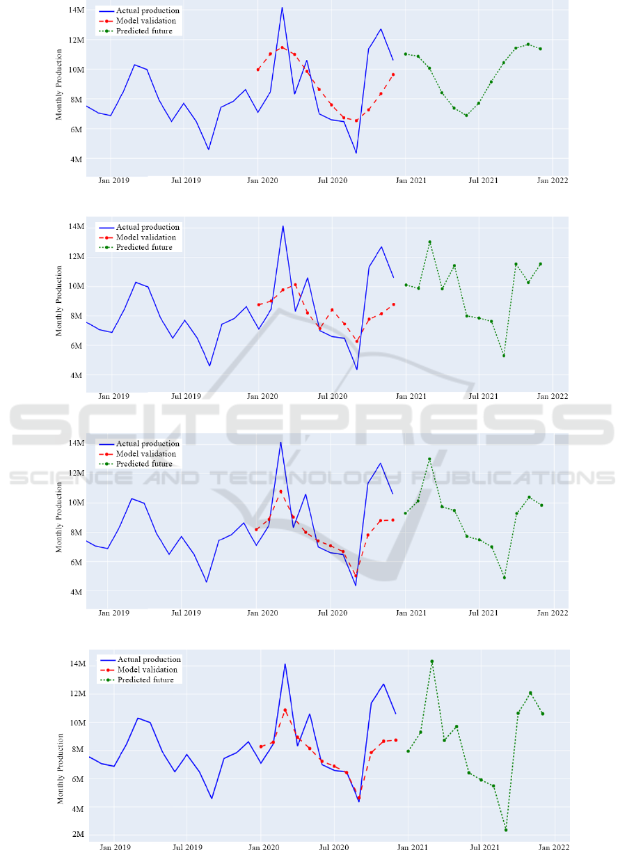
Figure 8: M1 results on product P1.

Figure 9: M2 results on P1.

Figure 10: M3 results on P1.

Figure 11: M4 results on P1.

NCTA 2023 - 15th International Conference on Neural Computation Theory and Applications

530

REFERENCES

Alkaabi, N. and Shakya, S. (2022). Comparing ml models

for food production forecasting. In Bramer, M. and

Stahl, F., editors, Artiﬁcial Intelligence XXXIX, pages

303–308, Cham. Springer International Publishing.

Burden, F. and Winkler, D. (2009). Bayesian Regulariza-

tion of Neural Networks, pages 23–42. Humana Press,

Totowa, NJ.

Chai, T. and Draxler, R. (2014). Root mean square er-

ror (rmse) or mean absolute error (mae)?– arguments

against avoiding rmse in the literature. Geoscientiﬁc

Model Development, 7:1247–1250.

Fischer, T. and Krauss, C. (2018). Deep learning with long

short-term memory networks for ﬁnancial market pre-

dictions. European Journal of Operational Research,

270(2):654–669.

Hochreiter, S. and Schmidhuber, J. (1997). Long Short-

Term Memory. Neural Computation, 9(8):1735–1780.

Jose, J. (2022). Introduction to time series analysis and its

applications.

Kamran, M., Naqvi, S., Akram, T., Umar, H. G., Shahzad,

A., Sial, M., Khaliq, S., and Kamran, M. (2019). Lstm

neural network based forecasting model for wheat

production in pakistan. Agronomy, 9:72.

Kingma, D. and Ba, J. (2014). Adam: A method for

stochastic optimization. International Conference on

Learning Representations.

Liu, Y., Wang, Y., and Zhang, J. (2012). New machine

learning algorithm: Random forest. In Liu, B., Ma,

M., and Chang, J., editors, Information Computing

and Applications, pages 246–252, Berlin, Heidelberg.

Springer Berlin Heidelberg.

Livieris, I., Pintelas, E., and Pintelas, P. (2020). A cnn-lstm

model for gold price time series forecasting. Neural

Computing and Applications, 32.

Louhichi, K., Jacquet, F., and Butault, J.-P. (2012). Estimat-

ing input allocation from heterogeneous data sources:

A comparison of alternative estimation approaches.

Agricultural Economics Review, 13.

Mahmud, A. and Mohammed, A. (2021). A Survey on Deep

Learning for Time-Series Forecasting, pages 365–392.

Peng, J., Lee, K., and Ingersoll, G. (2002). An introduction

to logistic regression analysis and reporting. Journal

of Educational Research - J EDUC RES, 96:3–14.

Sagheer, A. and Kotb, M. (2019). Time series forecasting of

petroleum production using deep lstm recurrent net-

works. Neurocomputing, 323:203–213.

Salehinejad, H., Sankar, S., Barfett, J., Colak, E., and

Valaee, S. (2017). Recent advances in recurrent neural

networks.

Schober, P., Boer, C., and Schwarte, L. (2018). Correla-

tion coefﬁcients: Appropriate use and interpretation.

Anesthesia & Analgesia, 126:1.

Shumway, R. and Stoffer, D. (2017). Time Series and Its

Applications.

Ullrich, T. (2021). On the autoregressive time series

model using real and complex analysis. Forecasting,

3(4):716–728.

Van Houdt, G., Mosquera, C., and N

apoles, G. (2020). A

review on the long short-term memory model. Artiﬁ-

cial Intelligence Review, 53.

Vaswani, A., Shazeer, N., Parmar, N., Uszkoreit, J., Jones,

L., Gomez, A. N., Kaiser, L. u., and Polosukhin,

I. (2017). Attention is all you need. In Guyon,

I., Luxburg, U. V., Bengio, S., Wallach, H., Fer-

gus, R., Vishwanathan, S., and Garnett, R., editors,

Advances in Neural Information Processing Systems,

volume 30. Curran Associates, Inc.

Testing Variants of LSTM Networks for a Production Forecasting Problem

531