Learning Based Interpretable End-to-End Control Using Camera Images

Sandesh Athni Hiremath, Praveen Kumar Gummadi, Argtim Tika, Petrit Rama and Naim Bajcinca

Department of Mechanical and Process Engineering, Rheinland-Pf

alzische Technische Universit

at Kaiserslautern-Landau,

Gottileb-Daimler-Straße 42, 67663 Kaiserslautern, Germany

Keywords:

Autonomous Driving, MPC, Learning Based Control, End-to-End Control, Lane Detection.

Abstract:

This work proposes a learning-based controller for an autonomous vehicle to follow lanes on highways

and motorways. The controller is designed as an interpretable deep neural network (DNN) that takes as

input only a single image from the front-facing camera of an autonomous vehicle. To this end, we ﬁrst

implement an image-based model predictive controller (MPC) using a DNN, which takes as input 2D

coordinates of the reference path made available as image pixels coordinates. Consequently, the DNN based

controller can be seamlessly integrated with the perception and planner network to ﬁnally yield an end-to-end

interpretable learning-based controller. Here, all of the controller components, namely- perception, planner,

state estimation, and control synthesizer, are differentiable and thus capable of active and event-triggered

adaptive training of the relevant components. The implemented network is tested in the CARLA simulation

framework and then deployed in a real vehicle to ﬁnally demonstrate and validate its performance.

1 INTRODUCTION

An autonomous driving system consists of various

sub-systems, starting from environment perception,

localization, scene understanding, decision-making,

and controller (Thrun et al., 2006). Every sub-

system outputs intermediate results and representa-

tions, which are very important for tracing decisions,

interpretation, and improving the overall performance

of the system. However, this approach is often time-

consuming and also lacks global consistency, as mod-

ules are optimised for intermediate results rather than

the end task. To remedy this, inspired by the works

of (Pomerleau, 1988) (T. Jochem and D. Pomerleau,

1995) (LeCun et al., 2005) and driven by recent ad-

vancements in data-driven and deep learning meth-

ods (Bojarski et al., 2016) (Codevilla et al., 2019)

(Bansal et al., 2019) (Natan and Miura, 2023), re-

searchers are focusing on developing robust end-to-

end approaches, where all modules are optimized for

the end task. One major issue that arises in end-

to-end approaches is the lack of explainability and

interpretability of intermediate outputs. The recent

learning-based approaches that dominate the method-

ology for implementing end-to-end algorithms suffer

from this problem.

Modular approaches, such as conventional solu-

tions, have the advantage of interpretability for each

involved sub-modules, thus useful for fault detection

in case of unexpected system behavior. Although the

sub-modules are developed separately, they are tightly

coupled and interdependent. Hence, it demands do-

main expertise and additional time to integrate and

maintain the whole pipeline. In autonomous driv-

ing, this is especially the case for perception, data fu-

sion, and localization modules. An overview cover-

ing these modules, their technical and functional as-

pects, as well as the main challenges, is presented in

(Velasco-Hern

andez et al., 2020). On the other hand,

an overview of approaches and challenges about plan-

ning and decision-making modules for self-driving

vehicles, is presented in (Schwarting et al., 2018).

Although control modules can be realized inde-

pendently or jointly as a single integrated framework

with the path planning, they are nonetheless tightly

coupled with the perception and state estimation lay-

ers. This makes it challenging to obtain a generalized

and robust system behavior. As an optimization-based

control technique, model predictive control (MPC) is

widely used in automated systems to plan an opti-

mal trajectory or follow a given reference path. MPC

exhibits high structural ﬂexibility in deﬁning qual-

ity and target criteria by means of a cost function

and state/input constraints. These jointly ensure that

system-relevant limits are adhered to, thus ensuring

safe operation. Focusing on path tracking for au-

tomated road vehicles, (Stano et al., 2022) provides

a comprehensive overview and classiﬁcation of dif-

474

Hiremath, S., Gummadi, P., Tika, A., Rama, P. and Bajcinca, N.

Learning Based Interpretable End-to-End Control Using Camera Images.

DOI: 10.5220/0012206500003543

In Proceedings of the 20th International Conference on Informatics in Control, Automation and Robotics (ICINCO 2023) - Volume 1, pages 474-484

ISBN: 978-989-758-670-5; ISSN: 2184-2809

ferent MPC formulations published in recent years.

Particularly in autonomous driving, many researchers

make use of MPC for path planning or path following

control (Paden et al., 2016) (Weiskircher et al., 2017)

(Ji et al., 2017) (Alcala et al., 2020). The proposed

algorithms are validated mainly by simulations, con-

sidering different driving scenarios. In (Kim et al.,

2021), an MPC-based approach with a variable pre-

diction horizon is proposed, where experiments with

a real vehicle at low speed are performed in addition

to simulations in CARLA. A learning-based MPC us-

ing Gaussian process regression to improve the vehi-

cle model online is presented in (Kabzan et al., 2019)

and tested on the AMZ race car (Kabzan et al., 2020).

Compared to modular methods, end-to-end ap-

proaches solve the problem of autonomous driving as

a single module, from feature extraction/engineering

to decision-making and control algorithms. This ap-

proach maps input data from the vehicle’s sensors to

the output of low-level control commands, such as

steering, braking, and acceleration. The overall archi-

tecture is uniﬁed and acts as a black box without sub-

modules and intermediate outputs. However, due to a

lack of meaningful intermediate outputs, the system’s

explainability is lower, and therefore harder to trace

its decision or the root cause of an error. Moreover,

this approach raises challenges such as the require-

ment of bigger models, thus larger computation over-

head, for obtaining sufﬁciently robust encoded fea-

tures and for fusing information across different sen-

sor modalities.

One of the earliest neural networks, ALVINN, dat-

ing back to 1989, was trained end-to-end for predict-

ing steering angle from camera and radar images for

the task of lane following on public roads without

human intervention (Pomerleau, 1988). In 1995, a

project named “No Hands Across America” was pro-

posed, training an end-to-end model for lane keeping,

mapping video images to steering angle, assisted by a

human driver to control the acceleration and braking

of the vehicle (T. Jochem and D. Pomerleau, 1995).

DAVE, a small robot car, was proposed to avoid ob-

stacles and navigate using image inputs. It also was

trained as an end-to-end convolutional neural network

(CNN) to predict steering angles for off-road vehicle

control (LeCun et al., 2005). End-to-end approaches

came again in prominence when NVIDIA proposed

a large-scale CNN for learning meaningful road fea-

tures in order to solve the entire task of lane following

by steering the vehicle in different environments and

weather conditions (Bojarski et al., 2016). Another

end-to-end algorithm is introduced in (Hecker et al.,

2018) to learn low-level car maneuvers from realistic

inputs of surround-view cameras. More recently, in

(Xiao et al., 2023), the authors have used CNN and

long short-term memory (LSTM) along with a differ-

entiable control barrier network for vision-based end-

to-end autonomous driving. However, it relies on the

availability of a nominal controller that generates fea-

sible controls.

Another simple form of end-to-end learning is

imitation learning (IL), an approach for training au-

tonomous driving systems by imitating an expert hu-

man driver, i.e., steering, acceleration, or braking

(Codevilla et al., 2019). Although it works well

for simple scenarios of lane following, this approach

faces difﬁculties in complex trafﬁc scenarios since us-

ing just the image as an input is not enough to predict

high-level maneuvers or to map the input into low-

level vehicle control commands. To address these

problems, conditional IL is introduced in (Codevilla

et al., 2018) by mapping the input of the planned ma-

neuver, apart from the perception input, into the con-

trol signal of steering angle and acceleration at train-

ing time. Planned maneuvers are also used as an in-

put in (Xiao et al., 2022), experimenting with multi-

modality of perception data and different stages of

data fusion for conditional IL. A further IL framework

is presented in (Bansal et al., 2019) by synthesizing

trajectory perturbation and augmenting undesirable

behavior to increase the robustness of the model. It is

also worth mentioning the interesting work of (Chen

et al., 2022), where a Bayesian interpreted reinforce-

ment learning (RL) method is proposed for end-to-

end learning in urban scenarios. This, however, in-

volves latent variables which are difﬁcult to physi-

cally interpret thus troublesome for debugging.

Taking advantage of both approaches, we pro-

pose a novel end-to-end approach in which percep-

tion, planning, state estimation, and control modules

are implemented in a differentiable manner via the use

of DNNs. As a result, we retain the interpretability

of intermediate outputs and gain robustness of DNNs

and tuning ﬂexibility to meet global system perfor-

mance. This end-to-end learnable and interpretable

framework takes images as input, and produces con-

trols and future trajectories of the ego-vehicle as out-

puts. The perception module detects static features

of the road in the form of lane markings and deliv-

ers them as the primary information for navigation.

The intermediate output from the perception module

and planner serves as a candidate reference target for

the controller, thus interpretable. The feedback (state

estimation) layer not only ﬁlters out a suitable tra-

jectory for the ego-vehicle but also estimates the ve-

hicle’s current state. Altogether, the involved mod-

ules, namely- lane detection, planning, state estima-

tion, and controller, are jointly optimizable for the end

Learning Based Interpretable End-to-End Control Using Camera Images

475

task of lane following. The developed model is vali-

dated by testing on a real vehicle.

The remainder of the paper is organized as fol-

lows. The addressed problem is deﬁned in Sec. 2. The

proposed end-to-end control approach, including all

its components, is described in Sec. 3. Sec. 4 presents

the implementation architecture and experimentation

results. In Sec 5, we discuss the results and provide

some concluding remarks.

2 PROBLEM DEFINITION

In this work, we consider the problem of lane follow-

ing by an autonomous vehicle equipped with a sin-

gle front-facing camera. To this end, we ﬁrst provide

an MPC formulation, which on one hand, serves as

a mathematical representation of the lane following

task, and on the other hand, serves as a foundation for

developing an end-to-end learning-based controller.

Let X ∈ R

, U ∈ R

, Y ∈ R

denote the

state, control and output variables, respectively,

of a dynamical system and expressed with respect

to (w.r.t) O

, the vehicle coordinate system. Let

F : R

× R

→ R

and H : R

× R

→ R

be C

functions, i.e. continuously differentiable functions.

Based on this let the dynamics of the system be

speciﬁed by

X(t) = F(X(t),U(t)), t > 0,

Y (t) = H(X(t),U (t)), t ≥ 0,

X(0) = x.

(1)

Let X , Y , and U denote the sets of admissible states,

outputs, and controls, respectively. Let Y(t) ∈ Y de-

note the target path of the vehicle and G(t) ∈ G denote

the environmental constraints on the vehicle, then the

path following problem can be posed as the task of

ﬁnding an optimal control U(t) ∈ U such that the ve-

hicle with the current state x reaches the target path

Y(t) ∈ Y while adhering to the environmental con-

straint G(t) ∈ G in the ﬁxed time horizon [t,t + T

t,T

> 0. Mathematically, this can be formulated as

the following optimal control problem (OCP):

J(X,U; Y) =

sλ

∥H(X,U) − Y(s)∥

sλ

∥U(t + s)∥

ds,

∗

(t),U

∗

(t) = argmin

X∈X ,U∈U

J(X,U; Y),

(t + s) = F(X (t + s),U(t + s)),s ∈ (0, T

]

X(t) = x(t), X(t + s) ≤ G(t + s).

(2)

Solving (2) for each time step t using the data

Y(t),G(t) and x(t) obtained from planning, percep-

tion and feedback modules, respectively, we obtain

the standard MPC algorithm. Thus, the general se-

quence of steps required to solve the lane following

task are (i) perceive, (ii) plan, and (iii) control. Since,

as mentioned above, we are interested in devising an

end-to-end learning based algorithm and also offering

good interpretability of outputs, we design each of the

above mentioned modules as neural networks. The

designed networks are such that when combined, they

form a single computational chain. Consequently, it

facilitates back-propagation of the prediction errors

up to the input layer, thereby enabling end-to-end,

i.e., output-to-input learning mechanism. To this end,

we have implemented four neural networks, which are

then combined together to obtain a single end-to-end

interpretable image-based controller network, which

we refer to as the EyeCon network (shortly as Eye-

ConNet). The ﬁrst two components of EyeConNet

are the camera based lane-detection and virtual trajec-

tory generation (VTG) networks, named together as

LDVTG. The next (third) component is the feedback

network (shortly as FB) which provides the mecha-

nism for estimating the state of the vehicle based on

the features obtained from the input camera image,

mainly from the output of the LDVTG. Finally, the

fourth component is the controller network, called the

VehCon, which serves as the model predictive con-

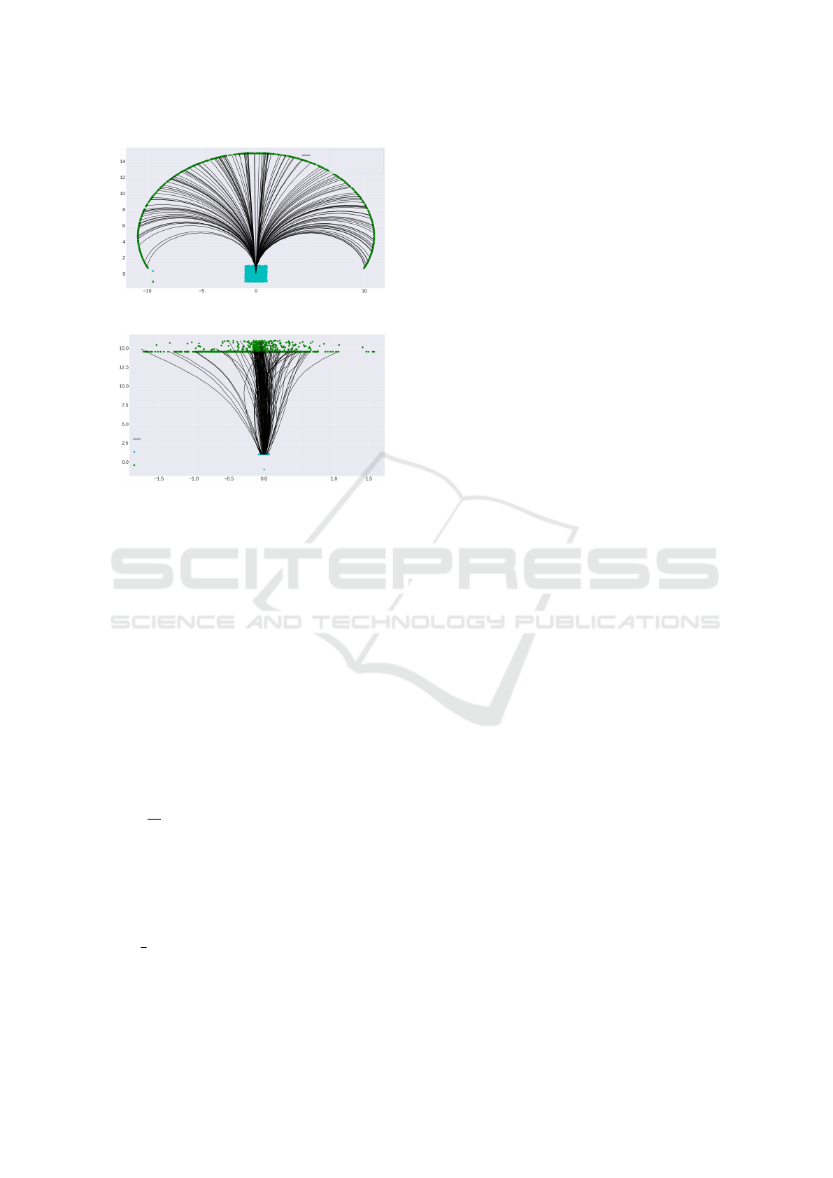
troller. Altogether, combining the four, as depicted in

Fig. 3, yields an interpretable network for the task of

following the lane by using only a single front-facing

camera. To the best of our knowledge, the proposed

approach for designing a tuneable autonomous con-

troller that uses only a camera image as the input and

whose behavior is validated on a real vehicle and real

roads has not been made before.

3 COMPONENTS OF THE EyeCon

NETWORK

3.1 Perception and Planning Network

The core perception task for lane following is lane

detection. To this end, we rely on the existing

work of Ultra Fast Structure-aware Deep Lane Detec-

tion (UFLD) (Qin et al., 2020). Although it works

quite well on regular RGB images, it showed poor

performance on images obtained from our vehicle.

The UFLD model trained on TuSimple dataset (TuS,

2023) (even with CuLane and CurveLanes dataset)

did not provide stable and continuous lane detection

across the frames obtained from our test vehicle. We

ICINCO 2023 - 20th International Conference on Informatics in Control, Automation and Robotics

476

argue that the reason for this is the difference in cam-

era settings (i.e., high saturation, brightness, etc.) be-

tween the camera from our test vehicle and the camera

used to obtain the images of the TuSimple dataset. To

overcome this problem, we collected and labeled ap-

proximately 1200 images with the front-facing cam-

era of our test vehicle and used them to ﬁne-tune the

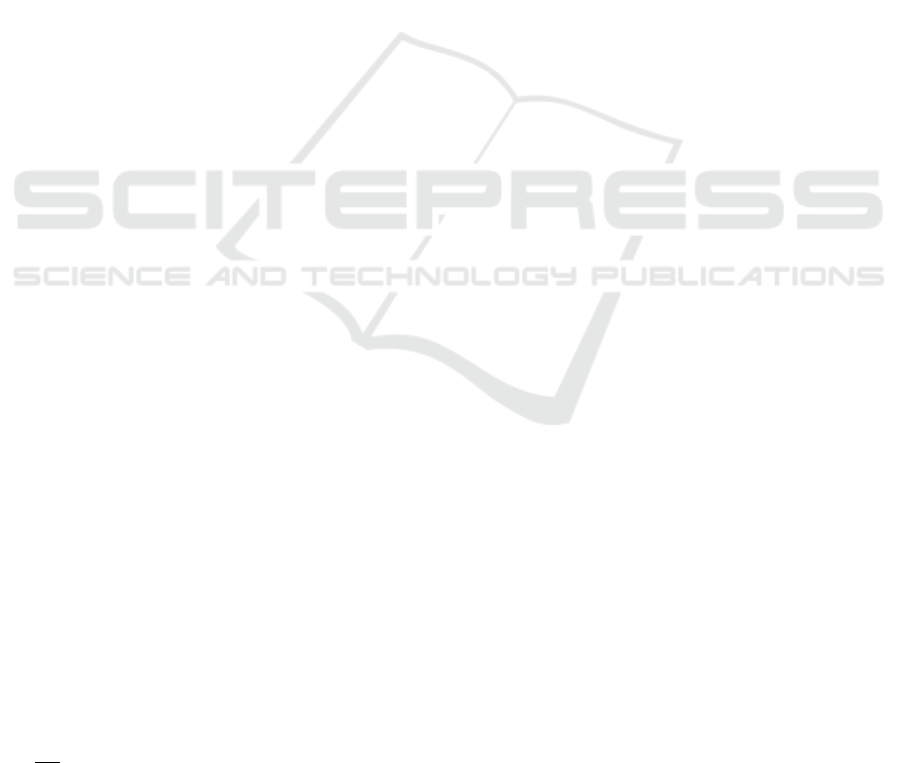
model. After this step, as evident in Fig. 1, the detec-

tions were consistent and stable across video frames

obtained while driving.

Since UFLD outputs detection probabilities across

downscaled columns for four lanes and for ﬁxed row

anchor positions, in order to obtain lane and trajectory

coordinates, we introduce two custom layers that con-

stitute the VTG network (or layer). The algorithmic

steps of VTG network (or layer) are as follows: (i)

for each row and lane-type ﬁlter out low probability

detections, (ii) do a softmax across columns and scale

it (based on image resolution) to obtain column posi-

tion, (iii) sort the tensor based on a reverse ordering

of row index, so that the bottom-most pixel (denoting

near ﬁeld) is ﬁrst, while the top most pixel (denoting

far ﬁeld) is last, and ﬁnally (iv) resample the tensor

to have ﬁxed number of pixels for each of the four

lanes. Based on the ﬁxed number of lane coordinates

for each lane, we perform the weighted sum of ad-

jacent lane coordinates to obtain the lane-following

trajectory. Consequently, the output of VTG is four

lanes and three trajectory coordinates. The above-

mentioned operations are implemented in a differen-

tiable manner and without disrupting the computation

graph.

3.2 Controller

In this section, we introduce a novel learning based

control algorithm for the problem of lane follow-

ing. We rely on the above MPC formulation based

on the OCP (2) to achieve this. Accordingly, given

x := (x,Y, G), where x is the current state of the vehi-

cle, Y is the reference trajectory and G is the environ-

mental constraints, the solution U

∗

to the OCP (2) can

be written as a mapping x 7→ M (x) with U

∗

:= M(x).

From this perspective, a practically convenient way

to implement a learning based controller is to train

a DNN to learn the mapping x 7→ M(x). We do so

via the following steps: (i) we set up a kinematic

model, which serves as a prediction (state propaga-

tion) model, and (ii) we implement a network for the

generation of optimal controls.

3.2.1 Vehicle Kinematic Model (VKM)

The motion of the vehicle on a 2D road is modeled

at the kinematic level so that the network is easily

(a) Detected lanes by UFLD.

(b) Ego lanes and trajectory.

Figure 1: Outputs from UFLD (left image) and the VTG

(right image). The left image shows the detected lanes of

UFLD after training on TuSimple (orange) and ﬁne-tuning

on RPTU (dark purple) datasets, respectively. The right im-

age shows the ego lane (dark purple) and the generated ego

trajectory (green).

generalizable and thus be applicable to any nonholo-

nomic front axle steered vehicles. Since we are inter-

ested in trajectory tracking, we follow the approach of

(Weiskircher et al., 2017) to model the kinematics in

the Frenet coordinate system given by the prescribed

trajectory. Following this, the error dynamics of the

vehicle is expressed in the Frenet frame O

of the ref-

erence path. Letting ψ

and ψ

denote the orienta-

tion of the reference frame and course angle of the

vehicle, the yaw-error ψ

is deﬁned as ψ

= ψ

− ψ

The distance of the vehicle to the reference path along

denotes the lateral distance and thus represents the

lateral error of the vehicle w.r.t the reference path.

Its dynamics is given as: ˙y

= v

sin(ψ

) where v

is the instantaneous velocity experienced at the ve-

hicle’s center of gravity (CoG). Similarly, the yaw-

error dynamics

can be given as:

− ˙sκ

with ˙s = v

cos(ψ

)(

1−y

). Here, s denotes the length

along the reference trajectory and κ = 1/ρ denotes the

curvature of the reference path, with ρ being the ra-

dius of the circle of instantaneous rotation (CIR). In-

troducing the control variables a

and α, which denote

longitudinal acceleration and yaw rate of the CoG re-

spectively, the dynamics of the planar motion of the

Learning Based Interpretable End-to-End Control Using Camera Images

477

vehicle is given by the equations:

˙y

= v

sin(ψ

= α

−

cos(ψ

)κ

(1 − y

κ)

˙v

= a

= α, ˙s =

cos(ψ

)

(1 − y

κ)

, (3)

˙x = v

cos(ψ

), ˙y = v

sin(ψ

Let U = [a

,α]

⊤

∈ R

denote the control vector and

X = [X

,. .. ,X

]

⊤

= [v

,ψ

,s, ψ

,x, y]

⊤

∈ R

denote the state vector of the vehicle, the VKM can

be compactly written in the form of (3) where H is a

suitable matrix such that

H(X,U) = H(X ) = [v

,ψ

,x, y]

⊤

∈ R

Based on this and denoting s := {e,c, p,dc, d p}, the

cost function J for the associated MPC formulation

reads as

J(X,U; Y) = γ

(X) + γ

(X,Y) + γ

(U)

+ γ

d p

(X) + γ

(U), (4)

(X) =

−1

∑

n=1

nλ

∥X

)∥

+ λ

∥X

)∥

(U) =

−1

∑

n=1

nλ

∥U

∥

+ λ

∥U(t

)∥

(X,Y) =

−1

∑

n=2

nλ

∥X

) − Y(t

)∥

+ λ

∥X

) − Y(t

)∥

d p

(X) =

∑

n=2

nλ

∥X(t

) − X(t

n−1

)∥

d p

(U) =

∑

n=2

nλ

∥U(t

) −U(t

n−1

)∥

where, N

∈ N is the number of discrete points for

the time horizon [t,t +T

], t

= t +

, X

= [ψ

]

⊤

denotes the error vector, X

= [v

,x, y]

⊤

denotes the

tangential speed and position vector. The quantities

for j ∈ s, denotes the scaling factor and

weighting matrices for the loss terms.

3.2.2 Network Architecture

The controller network (VehCon) is designed as

a stacked recurrent network composed of Gated-

Recurrent-Units (GRUs). An i-th GRU cell, N

takes as input the i-th component of the input-data Y

and G

to generate the estimate

, which is then fed

to N

, a fully connected network whose weights are

shared across temporal points, to obtain the control

for i-th time step. The output of the network is the

sequence of controls

U and the states

X predicted by

the controls. Since the control network is designed to

play the role of a statistical optimizer, its loss func-

tional L is based on J (4) and is given as

L(X,U,Y) := L(X,U, Y) + γ

(X,U,Y),

L(X,U,Y) := J(X ,U; Y), (5)

(X,G) :=

+ ∥X − G∥

, ε

:= .001,

(X,U,Y) := ρ([L

]

⊤

= diag([q

]

⊤

), Q

= diag([q

]

⊤

= diag([q

]

⊤

), Λ = [λ, λ

,λ

]

⊤

where, L

is acting as a barrier function that han-

dles environmental constraints, ρ is a parameterized

robust-loss-functional (Barron, 2019). Altogether, the

VehCon is composed of 174 K learning parameters

that amounts to 837 KB of memory consumption.

Next, the data required for training the statistical opti-

mization solver is synthetically generated by appro-

priately sampling the inputs from the valid range.

Based on this x ∈ U([−1, 1]), Y a local trajectory

for the vehicle, is obtained by parameterizing with

respect to the curvature κ, which is uniformly sam-

pled from [−.1, .1]. The generated trajectories are set

to have lane-boundaries at ﬁxed lateral distances. In

this manner, we generate a generic dataset to cover

all possible (local) maneuvers of the vehicle. Further-

more, we also collect the reference trajectories and

feedback input predicted by the LDVTG and FB net-

works on the RPTU test dataset. The former serves

for robust stand-alone training of the control network,

while the latter serves for ﬁne-tuning it on the outputs

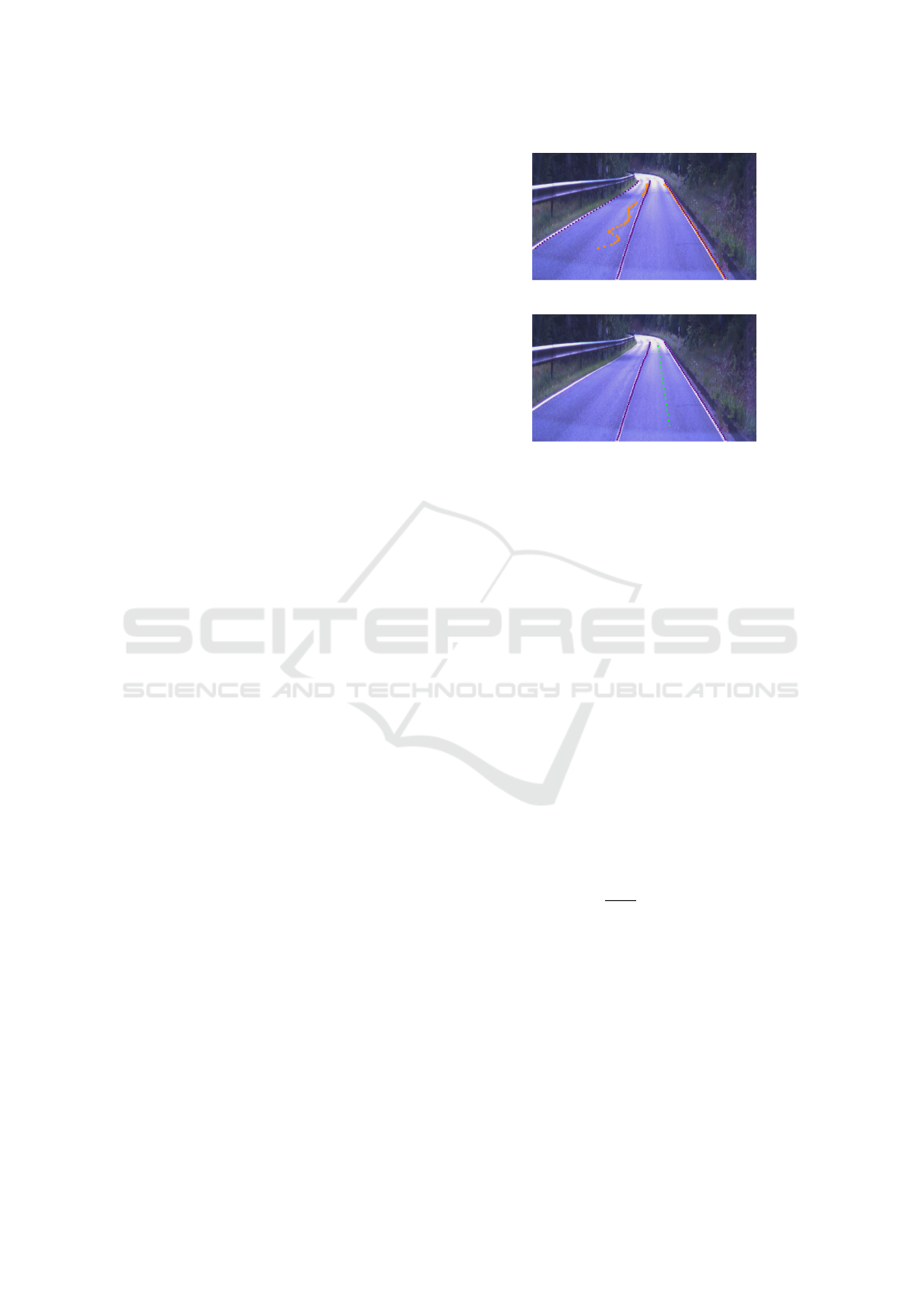
of the preceding components of the EyeConNet. Both

datasets are as shown in Fig. 2.

3.3 Feedback Network

The feedback network or layer (FB) is an important

component of EyeConNet that is responsible for esti-

mating the current state of the vehicle using only the

information obtained from the image features. The

feedback layer takes as input the lane and trajectory

coordinates (i.e. the output of VTG) and provides as

output (i) the ego reference and lane coordinates and

(ii) an estimate of the current vehicle state

X(t). The

former is obtained by selecting the lane and trajec-

tory (triplet) having more than a required number of

coordinates, which then serve as the ego or reference

ICINCO 2023 - 20th International Conference on Informatics in Control, Automation and Robotics

478

Synthetic dataset

x (m)

y (m)

Reference path

Start position

Target position

(a) Training samples.

x (m)

y (m)

RPTU dataset

Reference path

Start position

Target position

(b) RPTU data samples.

Figure 2: Samples from dataset consisting of reference

trajectories (black), start positions (cyan) and target end

(green) positions.

(triplet) coordinates. In this way, FB is also acting as

a naive decision-making layer. Once the ego triplet,

consisting of a pair of lane coordinates and reference

trajectory coordinates, are obtained, the ego trajec-

tory is used to estimate the state vector

X(t). Firstly,

since we want to generate the trajectory local to the

vehicle, we transform the pixels from the image co-

ordinate system to the vehicle coordinate system O

Consequently, this has the added beneﬁt that some of

the components of the state vector remain ﬁxed, i.e.

= π/2, ˆy = 0 and ˆx = −x

with x

:= 2m denot-

ing the ﬁxed look ahead distance of the camera. The

error components X

:= [y

(t),ψ

(t)]

⊤

is estimated

as follows. Let y

= (u

)

⊤

denote the i-th coordi-

nate of the ego trajectory in vehicle coordinate, then

ˆy

≈ −

∑

and

≈ −arctan([k

− u

]

⊤

)

with k

> 0 and k

≥ 1 acting as tuning parameters.

Based on testing and simulation we set k

= 5 and

= 2. Next, the curvature κ

(t) of the virtual tra-

jectory is obtained by using the parameterized curva-

ture formula, where derivatives are approximated by

ﬁnite differences. Based on this, the current estimate

X(t) of the vehicle state X at time t, w.r.t O

, is given

as [v

,0, ψ

,0, −x

]

⊤

. Here, v

is the open-loop

estimate of the vehicle velocity obtained by integrat-

ing (starting from the previous state) the acceleration

signal or from the IMU sensor. Similar to VTG, the

operations of FB are implemented in a differentiable

manner and do not consists of any learnable parame-

ters.

3.4 Training Methodology

To train the EyeConNet, we follow a three stage ap-

proach. In the ﬁrst stage (Stage1) we train the LD-

VTG, i.e., the UFLD and VTG networks, to obtain

stable lane detections and virtual trajectories. In the

second stage (Stage2) we use the predictions of the

LDVTG on the RPTU test-set as the training set and

ﬁnetune the VehCon. This is analogous to detach-

ing the computation graph of the VehCon from the

rest of EyeConNet while training. The parameters

involved in (4) and (5) for training the VehCon are

as described in Table 1. The Stage2 training mainly

facilitates in adapting the VehCon, which was pre-

trained on a generic vehicle kinematics dataset (see

Fig. 2), for the distribution of feedback inputs gen-

erated by the VTG. Subsequently, in the third stage

(Stage3) we combine VehCon and LDVTG to ob-

tain the EyeConNet, and train it on the combined

dataset of TuSimple and RPTU. For the uniﬁed train-

ing of EyeConNet, the learnable parameters of the

networks are the ones belonging to ULFD and Ve-

hCon, since, in the current implementation, the VTG

and FB do not have any learnable parameters. Based

on this, the loss function for the joint training is given

by L

EyeCon

= L

UFLD

+ 0.3L

VehCon

, where L

VehCon

given by (5) and L

UFLD

is as in (Qin et al., 2020).

The evaluation scores, on the joint test set of RPTU

and TuSimple, for each training stage are tabulated in

Table 2. For comparison, we have also mentioned the

baseline score obtained by using pretrained (TuSim-

ple) weights of the UFLD network. Firstly, the result

of Stage1 training (second row of Table 2) indicates

that both ﬁne-tuning (warm start) and fresh training

(cold start) of LDVTG network on the joint dataset do

not quantitatively alter the results much. However, as

depicted in Fig. 1, there is a signiﬁcant increase in the

quality in terms of pixel-wise and frame-wise conti-

nuity of the detected lanes on RPTU images. Next,

the result of Stage2 training (third row of Table 2)

is indicated by the RMSE value of the error vector

[ψ

] evaluated at the terminal time, t + T

, of the

prediction horizon. The obtained value of 0.123 is

small enough (i.e. y

< 15cm and ψ

< .1 degree) to

proceed with the next stage of training. Subsequently,

in Stage3 for training the EyeConNet we used the pre-

trained weights of the VehCon from Stage2. Here,

we performed experiments by warm starting and cold

starting the LDVTG, wherein the former uses the

baseline weights or starts fresh. Additionally, we also

Learning Based Interpretable End-to-End Control Using Camera Images

479

EyeConNet

VTG

UFLD

...

lane3

VehCon

lane1

lane2

lane4

ego-left

ego

ego-right

Feedback Layer

...

Input Camera Image

softmax

lane1

lane2

lane3

lane4

ego

ego-left

ego-right

Ego-lanes

& trajectory

Detection

Probabilities

predicted trajectoryreference trajectory

n-1

0 1

1 2

nn-1

Figure 3: Network architecture of EyeConNet, an end-to-end lane following controller network.

Table 1: Parameter values relating to the loss function L (5).

λ = 0.02 λ

= 20 λ

= .5 q

= 10

= .05 q

= 10 q

= 2 q

= .01 q

= 5

= 1 γ

d p

= 1 γ

= 10

−3

= 10

−5

= .005 γ

= 10

−5

= 2

experimented by having the computation graph for

the controller network either detached or joined with

the rest of the network. The former is referred to as

Stage3.0, and the latter as Stage3.1. Based on the

evaluation scores of each training stage tabulated in

Table 2, we see that ﬁrstly, cold start training is bet-

ter than the warm start, i.e., using pretrained UFLD

weights (baseline) is not quantitatively advantageous.

Secondly, we notice that detached training of VehCon

ensures that LDVTG has almost the same perfor-

mance as that of the Stage1. This is to say that the risk

of deterioration of LDVTG due to multi-tasked train-

ing of EyeConNet is reduced to almost zero by having

the VehCon in detached mode while training. Conse-

quently, the result of VehCon for Stage3 is similar to

that of Stage2 with Stage3.0 showing slightly better

and the Stage3.1 slightly worse performance. Look-

ing at Fig. 5 and Fig. 6, we see that the generated con-

trols are well-behaved in the sense that the error states

[ψ

]

⊤

are smoothly reduced to zero along the pre-

diction horizon such that the error distribution at the

end of the prediction horizon has the mean value close

to zero. Furthermore, from Fig. 7, we can also infer

that generated acceleration and yaw rates are smooth

and decay to zero along the prediction horizon. These

qualitative properties, along with good prediction re-

sults from EyeConNet, as depicted in Fig. 4, assure

conﬁdence for deploying it on the vehicle and testing

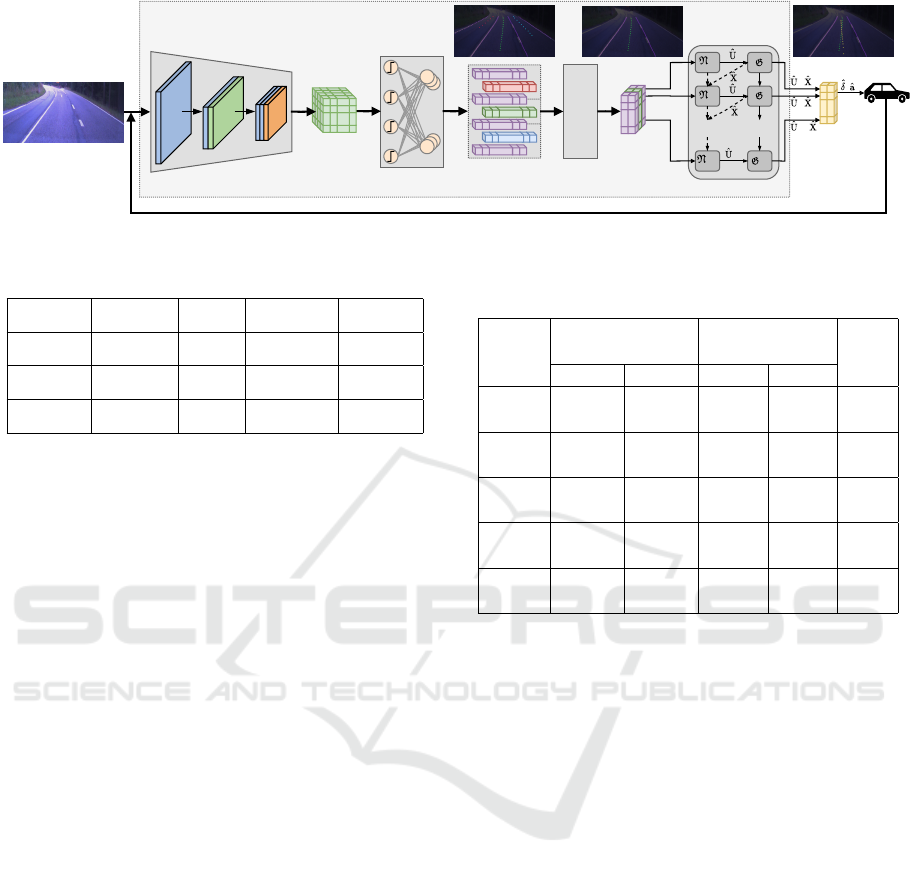
it on real scenarios.

Table 2: Stage wise training results for network compo-

nents.

Training

Fine Tuning Fresh Training

RMSE(warm start) (cold start)

Stages Acc F1-S Acc F1-S

Baseline 95.82% 87.88% - -

Stage1 95.60% 87.54% 95.27% 87.23% -

Stage2 - - - - 0.123

Stage3.0 95.6% 87.4% 95.8% 87.8% 0.118

Stage3.1 85.4% 62.5% 86.5% 66.4% 0.124

4 IMPLEMENTATION AND

RESULTS

The proposed algorithms are tested and validated on

an VW Passat, which has been modiﬁed to perform

autonomous driving experiments, see Fig. 8. The

experimental vehicle is equipped with power man-

agement, computational, environment sensing, and

communication resources, including CAN-bus-based

reading and writing access to the vehicle data, respec-

tively, vehicle actuators. In this work, perception is

based on a single camera directed toward the roadway.

The control algorithms are implemented in PYTHON

on a CarPC with NVIDIA A2 GPU and Intel Core i7-

8700T Processor with a clock rate of 2.40GHz. Since

EyeConNet is implemented using the PyTorch frame-

work, it was easily deployed in CarPC. Furhtermore,

to compare its performance, we also implemented the

standard MPC problem using the CasADi framework

(Andersson et al., 2019) and the resulting optimiza-

tion problem, i.e., the OCP (2), is solved with the

IPOPT solver (W

achter and Biegler, 2006).

A schematic of the lane following controller im-

plemented in the vehicle is shown in Fig. 9. The per-

ception module takes input from the camera and pro-

ICINCO 2023 - 20th International Conference on Informatics in Control, Automation and Robotics

480

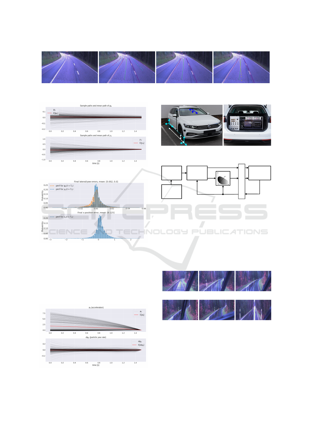
(a) Input Image. (b) Virtual trajectories. (c) Selected ego trajectory. (d) Predicted vehicle path.

Figure 4: Prediction result of EyeConNet on a sample test image.

Figure 5: Predicated error states ψ

and y

Figure 6: Error distributions of terminal position and orien-

tation of the vehicle.

vides the reference trajectory for the controller, which

then, following the idea presented in Section 3.2, syn-

thesizes optimal values for the vehicle longitudinal

acceleration ˆa

and the yaw rate

. The perception

block is nothing but the LDVTG, while the controller

block is the VehCon or a classical MPC-based con-

troller. Note that here we have, on purpose, decou-

Figure 7: Generated controls

Figure 8: Experimental vehicle.

ControllerPerception

Camera

Vehicle

ˆa

CAN

Figure 9: Schematics of the vehicle control architecture.

pled the perception and controller block to facilitate

the integration of the classical MPC with the LDVTG.

The controller takes the current velocity of the vehi-

cle as a feedback and uses it to update the state es-

timate from FB. Furthermore, the obtained yaw rate

is converted to the corresponding steering angle

δ using a three-dimensional function approximation

previously generated from measurements at different

vehicle speeds.

(a) Curve at sight (b) Entering curve (c) At curve

(d) Visual block (e) Exiting curve (f) Successful exit

Figure 10: Curve maneuver of EyeCon at 54 kmph under

poor visibility and heavy rain.

4.1 Results

In this section, we mainly focus on the experimen-

tal results performed with our experimental vehicle

VW Passat (see Fig. 8). Albeit, before proceeding

Learning Based Interpretable End-to-End Control Using Camera Images

481

to vehicle testing, we indeed tested EyeConNet in

CARLA for two different map environments namely

Town04 and Town06. In this test, the EyeConNet

was able to detect the lanes for more than 95% of the

frames and the detections were also sequentially sta-

ble. Consequently, the generated local trajectory was

always within the lane boundary and even centered.

As a result, the VehConNet was successful in follow-

ing the generated reference path successfully and re-

liably, which subsequently encouraged us to go ahead

with the real vehicle testing. For the real-world test-

ing, we performed tests on a public country-side road

that had sufﬁcient good lane markings. The tests are

performed for two target velocity speeds, 36km/h and

54km/h. For safety reasons, we have avoided testing

at higher speeds. In order to validate the perception

and planner module, i.e., the LDVTG, we also per-

form the same tests using a standard MPC controller.

This also serves as a comparison candidate for the Ve-

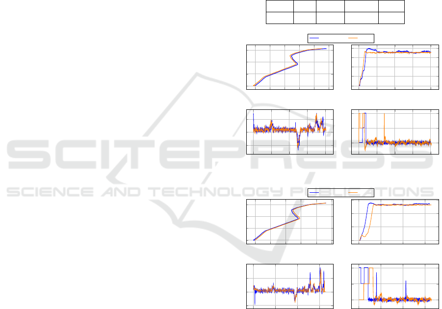
hCon. The obtained results are as depicted in Fig. 11.

Based on this, we can observe the following: (i) at the

global vehicle behavior level, both MPC and EyeCon-

Net based controllers were able to achieve the task

of lane following. The drive-experience was stable

and pleasant, without any abrupt behavior. The sta-

ble behavior of MPC indicates that LDVTG and FB

were sufﬁciently good in providing reliable lane de-

tections, reference trajectory, and state estimates. (ii)

The performance of the VehCon (DNN controller) is

in close comparison with that of the MPC. The tra-

versed trajectory in both cases was nearly identical

(as seen in the top left corner, blue vs. orange path)

for both target velocities. The high-level proﬁle of

the steering angle is also similar for both controllers.

This is to say that the turning maneuvers match each

other and also the road proﬁle. At higher speeds, the

magnitude of steering is relatively higher in compar-

ison to the lower speed. Furthermore, the VehCon is

more reactive to turns in the sense that it aligns to a

turn earlier and is thus marginally better at sharper

turns. Looking at the velocity proﬁles, we see that

both controllers are able to reach the respective tar-

get velocities pretty quickly and are able to maintain

it. However, the VehCon seems to be slightly aggres-

sive and tends to overshoot the reference. This is ex-

plainable from the control proﬁles generated by Ve-

hCon on the test set, which indicates a clear bias for

positive values, depicted in the upper plot of Fig. 7.

Despite this, we did not observe a deteriorating ef-

fect on the controller performance. Altogether, the

interpretable architecture of EyeConNet provides sat-

isfactory performance and offers robust validation and

testing mechanism. Furthermore, it also enabled the

computation time for each of the network components

to be measured during the closed loop operation of

the controller. This is tabulated in Table 3. As per

that, we see that perception and planning together take

under 15 ms in total, with perception being around

5 ms and planning around 9 ms, respectively, on av-

erage. The state estimation is even faster, with under

2 ms of runtime, while the control synthesizer takes

the most time, around 32.5 ms on average. Conse-

quently, all the modules combined, the total runtime

is under 50 ms, which we believe to be quite good for

the complexity of the task being considered.

Table 3: Mean computation times of network components.

UFLD VTG FB VehCon Total

5 ms 9 ms 1.5 ms 32.5 ms 48 ms

0 0.1 0.2 0.3 0.4 0.5

x (km)

y (km)

Vehicle path

EyeConNet MPC

0 50 100 150 200

Time (s)

(km/h)

Vehicle velocity

0 50 100 150 200

−0.25

0.25

Time (s)

δ (rad)

Steering angle

0 50 100 150 200

0.5

Time (s)

(m/s

)

Vehicle acceleration

(a) Results of experiment with 36 kmph as target velocity.

0 0.1 0.2 0.3 0.4 0.5

x (km)

y (km)

Vehicle path

EyeConNet MPC

0 50 100 150

Time (s)

(km/h)

Vehicle velocity

0 50 100 150

−0.5

0.5

Time (s)

δ (rad)

Steering angle

0 50 100 150

0.5

Time (s)

(m/s

)

Vehicle acceleration

(b) Results of experiment with 54 kmph as target velocity.

Figure 11: Comparison of Vehicle performance at different

target speeds of 36kmph (10m/s) and 54kmph (15m/s) when

fed with VehCon and MPC derived controls respectively.

5 CONCLUSION

In this paper, we have proposed an end-to-end inter-

pretable image based DNN controller called EyeCon-

Net, capable of steering and accelerating the vehicle

ICINCO 2023 - 20th International Conference on Informatics in Control, Automation and Robotics

482

directly from the image information. The modular

and interpretable design of EyeConNet not only al-

lowed us to train it incrementally, keeping the perfor-

mance of the fused network equal to that of their stan-

dalone counterparts, but also allowed seamless inte-

gration with the classic MPC controller, enabling ro-

bust and comparative testing. The developed network

was initially tested in CARLA, then subsequently

tested on real public roads while adhering to safety

requirements. The obtained performance for EyeCon-

Net was satisfactory and in good comparison with

a classical MPC controller. The stable performance

of MPC, when fed with LDVTG outputs, reassures

the stable performance of the perception and planner

modules, thanks to stage-wise training and ﬁnetuning

on images obtained from vehicle-speciﬁc cameras.

Furthermore, testing during rainy weather and low

visibility conditions, both MPC and EyeConNet were

able to show respectable performance (see Fig. 10)

with minor deterioration, i.e., occasional deactivation

of the control interface due to lack of reference trajec-

tory due to failure of LDVTG. Lastly, a highly com-

petitive runtime of under 50 ms of EyeConNet, on the

one hand, encourages us to consider even more com-

plex models to increase robustness and, on the other

hand, to consider active-closed-loop learning with ei-

ther MPC or driver in the loop. The latter opens up a

lot of interesting research problems, especially in the

area of IL and RL.

ACKNOWLEDGEMENTS

This work was supported by the German Federal Min-

istry of Transport and Digital Infrastructure (BMDV)

within the scope of the project AORTA with the grant

number 01MM20002A.

REFERENCES

Tusimple: Tusimple benchmark. https://github.com/

TuSimple/tusimple-benchmark. Accessed: 2023-03-

15.

Alcala, E., Sename, O., Puig, V., and Quevedo, J. (2020).

Ts-mpc for autonomous vehicle using a learning ap-

proach. IFAC-PapersOnLine, 53(2):15110–15115.

21st IFAC World Congress.

Andersson, J. A. E., Gillis, J., Horn, G., Rawlings, J. B., and

Diehl, M. (2019). CasADi – A software framework

for nonlinear optimization and optimal control. Math-

ematical Programming Computation, 11(1):1–36.

Bansal, M., Krizhevsky, A., and Ogale, A. S. (2019). Chauf-

feurnet: Learning to drive by imitating the best and

synthesizing the worst. In Robotics: Science and Sys-

tems XV, University of Freiburg, Freiburg im Breisgau,

Germany, June 22-26, 2019.

Barron, J. T. (2019). A general and adaptive robust loss

function. CVPR.

Bojarski, M., Testa, D. D., and et al. (2016). End to end

learning for self-driving cars. CoRR, abs/1604.07316.

Chen, J., Li, S. E., and Tomizuka, M. (2022). Interpretable

end-to-end urban autonomous driving with latent deep

reinforcement learning. IEEE Transactions on Intelli-

gent Transportation Systems, 23(6):5068–5078.

Codevilla, F., M

uller, M., L

opez, A. M., Koltun, V., and

Dosovitskiy, A. (2018). End-to-end driving via condi-

tional imitation learning. In International Conference

on Robotics and Automation, ICRA, pages 1–9. IEEE.

Codevilla, F., Santana, E., L

opez, A. M., and Gaidon, A.

(2019). Exploring the limitations of behavior cloning

for autonomous driving. In International Conference

on Computer Vision, ICCV 2019, pages 9328–9337.

IEEE.

Hecker, S., Dai, D., and Gool, L. V. (2018). End-to-end

learning of driving models with surround-view cam-

eras and route planners. In European Conference on

Computer Vision, ECCV, volume 11211 of Lecture

Notes in Computer Science, pages 449–468. Springer.

Ji, J., Khajepour, A., Melek, W. W., and Huang, Y. (2017).

Path planning and tracking for vehicle collision avoid-

ance based on model predictive control with multicon-

straints. IEEE Transactions on Vehicular Technology,

66(2):952–964.

Kabzan, J., Hewing, L., Liniger, A., and Zeilinger, M. N.

(2019). Learning-based model predictive control for

autonomous racing. IEEE Robotics and Automation

Letters, 4(4):3363–3370.

Kabzan, J., Valls, M. I., and et al. (2020). Amz driverless:

The full autonomous racing system. Journal of Field

Robotics, 37(7):1267–1294.

Kim, M., Lee, D., Ahn, J., Kim, M., and Park, J. (2021).

Model predictive control method for autonomous ve-

hicles using time-varying and non-uniformly spaced

horizon. IEEE Access, 9:86475–86487.

LeCun, Y., Muller, U., and et al. (2005). Off-road obstacle

avoidance through end-to-end learning. In Advances

in Neural Information Processing Systems 18, NIPS,

pages 739–746.

Natan, O. and Miura, J. (2023). End-to-end autonomous

driving with semantic depth cloud mapping and multi-

agent. IEEE Trans. Intell. Veh., 8(1):557–571.

Paden, B.,

ap, M., and et al. (2016). A survey of motion

planning and control techniques for self-driving urban

vehicles. IEEE Transactions on Intelligent Vehicles,

Pomerleau, D. (1988). ALVINN: an autonomous land ve-

hicle in a neural network. In Touretzky, D. S., editor,

Advances in Neural Information Processing Systems

1, [NIPS Conference, Denver, Colorado, USA, 1988],

pages 305–313. Morgan Kaufmann.

Qin, Z., Wang, H., and Li, X. (2020). Ultra fast structure-

aware deep lane detection. In European Conference

on Computer Vision, pages 276–291. Springer.

Learning Based Interpretable End-to-End Control Using Camera Images

483

Schwarting, W., Alonso-Mora, J., and Rus, D. (2018). Plan-

ning and decision-making for autonomous vehicles.

Stano, P., Montanaro, U., and et al. (2022). Model predic-

tive path tracking control for automated road vehicles:

A review. Annual Reviews in Control.

T. Jochem and D. Pomerleau (1995). No hands across amer-

ica ofﬁcial press release. Carnegie Mellon University.

Thrun, S., Montemerlo, M., and et al. (2006). Stanley: The

robot that won the DARPA grand challenge. J. Field

Robotics, 23(9):661–692.

Velasco-Hern

andez, G. A., Yeong, D. J., Barry, J., and

Walsh, J. (2020). Autonomous driving architectures,

perception and data fusion: A review. In Nedevschi,

S., Potolea, R., and Slavescu, R. R., editors, 16th

IEEE International Conference on Intelligent Com-

puter Communication and Processing, ICCP 2020,

Cluj-Napoca, Romania, September 3-5, 2020, pages

315–321. IEEE.

Weiskircher, T., Wang, Q., and Ayalew, B. (2017). Pre-

dictive Guidance and Control Framework for (Semi-

)Autonomous Vehicles in Public Trafﬁc. IEEE Trans-

actions on Control Systems Technology, 25(6):2034–

2046.

achter, A. and Biegler, L. (2006). On the implemen-

tation of an interior-point ﬁlter line-search algorithm

for large-scale nonlinear programming. Mathematical

programming, 106:25–57.

Xiao, W., Wang, T.-H., and et al. (2023). Barriernet: Dif-

ferentiable control barrier functions for learning of

safe robot control. IEEE Transactions on Robotics,

39(3):2289–2307.

Xiao, Y., Codevilla, F., Gurram, A., Urfalioglu, O., and

opez, A. M. (2022). Multimodal end-to-end au-

tonomous driving. IEEE Trans. Intell. Transp. Syst.,

23(1):537–547.

ICINCO 2023 - 20th International Conference on Informatics in Control, Automation and Robotics

484