Bayesian State Estimation Using Constrained Zonotopes
Lenka Kukli
ˇ
sov
´
a Pavelkov
´
a
a
The Czech Academy of Sciences, Institute of Information Theory and Automation
Pod Vodarenskou vezi 4, Prague, Czech Republic
Keywords:
Stochastic Systems, Recursive State Estimation, Bounded Noise, Constrained Zonotope, State-Space Models,
Linear Systems, Approximate Estimation.
Abstract:
This paper proposes an approximate Bayesian recursive algorithm for the state estimation of a linear discrete
time stochastic state space model. The involved state and observation noises are assumed to be bounded
and uniformly distributed. The support of a posterior probability density function (pdf) is approximated by a
constrained zonotope of an adjustable complexity. The behaviour of the proposed algorithm is illustrated by
simulations and compared with other methods.
1 INTRODUCTION
State estimation or filtering has many applications in
contexts where either the states, or the observations,
or both, are constrained to particular sets. The con-
strained filtering applications are used for example in
problems of fault detection (Scott et al., 2016), robust
model predictive control (Sharma et al., 2018), esti-
mation in sensor networks (Ge et al., 2019) and in ap-
plications involving constrained dynamics in physical
processes (Simon and Simon, 2010).
Deterministic state estimation uses so called set
membership approaches. There, states are guaranteed
to be contained in a bounded set as orthotopes, paral-
lelotopes, zonotopes and and ellipsoids (Althoff and
Rath, 2021).
These geometric considerations are important also
in a Bayesian filtering involving constrained (typi-
cally uniformly distributed) stochastic state and ob-
servation noise processes (Combastel, 2016).
The main advantages of Bayesian filtering are (i)
the possibility to take account of the distribution of
the states within their constrained support sets (Shao
et al., 2010), (ii) the quantification of uncertainty in
the states (S
¨
arkk
¨
a, 2013), and (iii) the evaluation of
the optimality, in the sense of minimum Bayes’ risk,
of sequential estimation and decision-making, includ-
ing control design (K
´
arn
´
y et al., 2006). Moreover,
it has been shown that the deterministic approach is
a particular case of the Bayesian general framework
(Samada et al., 2023).
a
https://orcid.org/0000-0001-5290-2389
In the author’s previous work, a Bayesian state es-
timator was proposed that provides optimally approx-
imated state estimates within the class of uniform dis-
tributions on orthotopic support (Pavelkov
´
a and Jirsa,
2018) and within the class of uniform distributions on
parallelotopic support (Jirsa et al., 2019).
This paper aims to enhance the above mentioned
Bayesian state estimator (Pavelkov
´
a and Jirsa, 2018)
and (Jirsa et al., 2019) and get a more flexible ap-
proximation of the true distribution while preserving
the feasibility of the resulting algorithm. We achieve
this by the by considering the state estimates within a
constrained zonotopic support.
The class of constrained zonotopes (CZ) has been
proposed in (Scott et al., 2016) as a tool for set-based
estimation. CZ can describe arbitrary convex poly-
tope when the complexity of the representation is not
limited. At the same time, this representation al-
lows the computation of exact projections, intersec-
tions, and Minkowski sums using very simple identi-
ties. To keep the computations feasible, methods for
computing an enclosure of one CZ by another one
of lower complexity are provided (Raghuraman and
Koeln, 2022).
Set membership estimators based on CZ are pre-
sented e.g. in (Rego et al., 2020b) or (Pan et al.,
2022). In contrast, we will use CZ to design a
Bayesian estimator.
Throughout, I is the identity matrix, R
n
is the n-
dimensional real space. Matrices are denoted by cap-
ital letters (e.g. A), vectors and scalars by lowercase
letters (e.g. b). Vector inequalities, e.g. x < x are
Kuklišová Pavelková, L.
Bayesian State Estimation Using Constrained Zonotopes.
DOI: 10.5220/0012230900003543
In Proceedings of the 20th Inter national Conference on Informatics in Control, Automation and Robotics (ICINCO 2023) - Volume 2, pages 189-194
ISBN: 978-989-758-670-5; ISSN: 2184-2809
Copyright © 2023 by SCITEPRESS – Science and Technology Publications, Lda. Under CC license (CC BY-NC-ND 4.0)
189

meant entry-wise; x and x are lower and upper bounds
on x, respectively. ℓ
x
denotes the length of a (col-
umn) vector x, and X denotes the set of x. x
t
is the
value of a time-variant vector x, at a discrete time in-
stant, t ∈ T ≡ {1, 2,... ,t}; x(t) ≡ {x
t
,x
t−1
,. .. ,x
1
}.
The symbol f (·|·) denotes a conditional probability
density function (pdf); no notational distinction is
made between a random variable and its realisation.
U
x
(x, x) is the uniform pdf of x with an orthotopic
(box) support [x, x] and U
x
(X) denotes the uniform
pdf of x on a bounded convex set X.
2 ADDRESSED PROBLEM
In the Bayesian filtering framework (K
´
arn
´
y et al.,
2006), a system of interest is described by the fol-
lowing probability density functions (pdfs):
- prior pdf f (x
1
)
- observation model f (y
t
|x
t
), t ∈ T (1)
- time evolution model f (x
t+1
|x
t
,u
t
), t ∈ T \t
where y
t
∈ R
ℓ
y
is an observable output, u
t
∈ R
ℓ
u
is
an optional known (exogenous) system input and x
t
∈
R
ℓ
x
is an unobservable (hidden) system state.
Bayesian state estimation or filtering consists in
the evolution of the posterior pdf f (x
t
|d(t)) where
d(t) is a sequence of observed data records d
t
=
(y
t
,u
t
), t ∈ T. The evolution of f (x
t
|d(t) is described
by a two-steps recursion that starts from the prior pdf
f (x
1
) and ends with the data update at the final time
t = t:
• data update (Bayes’ rule) processing the new data
f (x
t
|d(t)) =
f (y
t
|x
t
) f (x
t
|d(t − 1))
R
X
t
f (y
t
|x
t
) f (x
t
|d(t − 1))dx
t
, (2)
• time update (marginalization) evolving the state at
the next time instant
f (x
t+1
|d(t)) =
Z
X
t
f (x
t+1
|u
t
,x
t
) f (x
t
|d(t)) dx
t
.
(3)
We consider that the stochastic system (1) is rep-
resented by a linear state-space model
y
t
= Cx
t
+ v
t
(4)
x
t+1
= Ax
t
+ Bu
t
+ w
t+1
with uniform prior pdf
x
1
= U
x
(x
1
,x
1
) (5)
where x
t
∈ R
ℓ
x
, y
t
∈ R
ℓ
y
, u
t
∈ R
ℓ
u
. A, B, C are known
model matrices of appropriate dimensions; v
t
and w
t
are additive random observational and modelling un-
certainties, respectively. We assume that v
t
and w
t
are mutually independent white noise processes uni-
formly distributed on known orthotopic supports:
f (v
t
) = U
v
(−ν,ν), f (w
t
) = U
w
(−ω,ω), (6)
where ν ∈ R
ℓ
y
, ω ∈ R
ℓ
x
.
We denote the linear state space model with uni-
form noises (4) – (6) as a LSU model.
The exact Bayesian state estimation of the LSU
model, according to (2) and (3) results in a non-
uniformly distributed posterior pdf on a geometrically
complex support.
To get applicable state estimation algorithm, two
points has to be addressed:
(i) In each data update step (2), the support of poste-
rior pdf corresponds to the intersection of the sup-
port from previous step and a strip given by new
data. To avoid computational complexity, the re-
sulting polytope is approximated in each step by
a tightly circumscribing orthotope in (Pavelkov
´
a
and Jirsa, 2018) or parallelotope in (Jirsa et al.,
2019). These approximations project the support
back to the initial class, i.e. the function is kept,
the support is changed.
(ii) In first time update step (3), the sum of two in-
dependent uniformly distributed random quanti-
ties results in a trapezoidal pdf (Kotz and Dorp,
2004), and each subsequent step further increases
functional complexity of the resulting pdf. To
preserve the class of the function and computa-
tional complexity, the trapezoidal pdf is approxi-
mated by a uniform pdf by minimising Kullback-
Leibler divergence of these pdfs (Pavelkov
´
a and
Jirsa, 2018). The result is a uniform pdf on the
support of the trapezoid, i.e. the support is kept,
the function is changed.
This paper will use the above mentioned approxi-
mation (ii) to keep the posterior pdf uniform and will
propose a more flexible approximation of its support,
using constrained zonotopes (Scott et al., 2016).
3 LSU-CZ FILTER
In this section, the constrained zonotopic (CZ) sets
are introduced and applied within the approximate
Bayesian state estimation (2) and (3) of LSU model
(4)–(6). The resulting constrained zonotopic state es-
timator is called LSU-CZ filter.
ICINCO 2023 - 20th International Conference on Informatics in Control, Automation and Robotics
190

3.1 Constrained Zonotopes
A zonotope is a centrally symmetric convex poly-
tope. It can be be described as the Minkowski sum
of a set of n
g
line segments, n
g
≥ n in n-dimensional
space. Zonotopes are often used to approximate com-
plex polytopes as their complexity can be easily tuned
and relevant set operations result in simple matrix cal-
culations (Combastel, 2015). Nevertheless, centrally
symmetric zonotopes are not suitable for tight ap-
proximation (circumscription) of generally asymmet-
ric convex polytopes. Therefore, a constrained zono-
tope (CZ) Z was introduced in (Scott et al., 2016):
Z =
{
Gξ + c : ∥ξ∥
∞
≤ 1, Aξ = b
}
≡
{
G,c, A,b
}
, (7)
where G ∈ R
n×n
g
is a generator matrix of rank n (with
n
g
generator columns vectors or generators), c ∈ R
n
is a zonotope centre and ξ ∈ R
n
g
, n
g
≥ n, A ∈ R
n
c
×n
g
and b ∈ R
n
c
, n
c
is a number of constraints (constrain-
ing equations in R
n
g
). Note that for n
g
= n linearly
independent generators with no constraints, Z is a par-
allelotope.
The following set operations are defined for
Z,U ⊂ R
n
, Y ⊂ R
k
, R ∈ R
k×n
:
RZ =
{
Rz : z ∈ Z
}
, (8)
Z + U =
{
z + u : z ∈ Z, u ∈ U
}
, (9)
Z ∩
R
Y =
{
z ∈ Z : Rz ∈ Y
}
, (10)
where (8) is a linear mapping of Z by R, (9) is the
Minkowski sum of sets Z and U and (10) is a general-
ized intersection of sets Z and Y. Note that for R = I
and k = n, a standard set intersection is obtained.
Applying to the constrained zonotopes, the opera-
tions (8), (9) and (10) result in (Scott et al., 2016):
RZ =
{
RG
z
,Rc
z
,A
z
,b
z
}
(11)
Z + U =

[G
z
G
u
],c
z
+c
u
,

A
z
0
0 A
u

,

b
z
b
u

, (12)
Z ∩
R
Y =



[G
z
0],c
z
,


A
z
0
0 A
y
RG
z
−G
y


,


b
z
b
y
c
y
−Rc
z





,
(13)
where subscripts z, u and y refer to the respective sets,
0 is a zero matrix of appropriate dimensions. The
lifted zonotope
z ∈
{
G,c, A,b
}
⇐⇒

z
0

=

G
A

,

c
−b

(14)
is an unconstrained zonotope, with n
c
added coordi-
nates fixed to zero.
The operations (12) and (13) on constrained zono-
topes increase their complexity, i.e. number of gen-
erators n
g
and constraints n
c
. To keep the complex-
ity within the given limits, reduction operations are
proposed in (Scott et al., 2016). These operations
either (i) preserve the set (rescaling, removing zero
columns in a lifted zonotope (14), zero constraints or
parallel generators (Raghuraman and Koeln, 2022))
or (ii) approximate the set by circumscription (reduc-
tion of least significant generators or constraints).
3.2 State Estimation on a CZ Support
As mentioned in Section 2, one iteration of the
Bayesian filtering task, applied to the LSU model (4)–
(6), consist of (i) the data update (2) that corresponds
to the intersection of two sets followed by an approx-
imation that pushes the support of posterior pdf back
to the chosen class, and (ii) the time update (3) fol-
lowed by an approximation of resulting non-uniform
pdf by the uniform one (Pavelkov
´
a and Jirsa, 2018),
(Jirsa et al., 2019).
Here, we propose a more flexible approximation
of the support of a posterior pdf f (x
t
|d(t)) in the data
update (2) using a CZ (7). The approximation within
the time update step is maintained.
We denote the support of posterior pdf f (x
t
|d(t))
(2) by the symbol X
t
and the support of the state pre-
dictor f (x
t+1
|d(t)) (3) by X
t|t−1
. The support of prior
pdf is denoted as X
1
.
3.2.1 Data Update
The data update (2) processes f (x
t
|d(t − 1)) (starting
from prior f (x
1
) in t = 1) together with f (y
t
|x
t
) given
by (4) and (6). The exact pdf is uniformly distributed
on a support X
t
that results from the intersection of a
support X
t|t−1
obtained during previous time update
(or X
1
in the first step) and a strip given by new data
(Pavelkov
´
a and Jirsa, 2018). For CZ support X
t
, using
(13), holds
X
t
= X
t|t−1
∩
C
(y
t
− V
t
), (15)
where V
t
is a support of f (v
t
).
An advantage of CZ is that the relevant intersec-
tion stays within CZ class after data update. Never-
theless, the number of generators n
g
and constraints
n
c
(7) continually increases. To maintain n
g
and n
c
below the required limits, the complexity reduction
operations (Scott et al., 2016) are applied as needed.
3.2.2 Time Update
The time update step (3) processes f (x
t
|d(t)) from
previous data update together with f (x
t+1
|x
t
,u
t
) given
Bayesian State Estimation Using Constrained Zonotopes
191

by (4) and (6). The exact pdf f (x
t+1
|d(t)) is non-
uniformly distributed on a CZ support X
t+1|t
. Using
the set operations (11), (12) gives
X
t+1|t
= AX
t
+ Bu
t
+ W
t
, (16)
where W
t
is a support of f (w
t
).
For the next step, the resulting non-uniform pdf
is approximated according to (Pavelkov
´
a and Jirsa,
2018) which results in uniform pdf with support (16).
3.3 Point Estimates
To use the state estimates for the prediction and con-
trol problems, we need a point estimate. In the case
of standard, i.e. unconstrained zonotope, its centre
can be chosen as the point estimate. When using con-
strained zonotope (7), the centre is not guaranteed to
be placed inside this set. Below, two ways of a choice
of the point estimate are proposed.
Method 1. The point estimate ˆx
1
corresponds to the
centre of an interval hull of the posterior pdf (15)
(Rego et al., 2020a).
Method 2. The point estimate ˆx
2
corresponds to the
point inside the posterior pdf (15) that is closest to the
centre of the relevant unconstrained zonotope. The
solution is obtained by solving two linear programs
(Raghuraman and Koeln, 2022).
3.4 Algorithmic Summary
The algorithmic sequence for LSUCZ filter is pro-
vided in Algorithm 1.
4 EXPERIMENTS
In this section, the proposed Algorithm 1 is compared
with the previous orthotopic (Pavelkov
´
a and Jirsa,
2018) and parallelotopic (Jirsa et al., 2019) variants.
4.1 Simulation Settings
The matrices of the state space model (4), (6) are set
as
A =


1.0 −0.5 0.2
0.5 0.1 0.0
0.3 0.0 −0.1


, B =


0.1
0.6
0.3


,
C =

1.0 0.0 0.5
0.0 1.0 0.5

,
Algorithm 1: State estimation with LSUCZ filter.
Initialization:
- set the initial time t = 1 and the final time t > 1
- set prior value of f (x
1
) (5)
- set noise parameters ν and ω in (6)
- set required maximal number of generators n
g
and
constraints n
c
for posterior (15)
Recursion: for t = 1, . . . , t − 1 do
I. Data update:
process d
t
into f (x
t
|d(t)) via (15)
II. Point estimate:
compute ˆx
i
,i = {1, 2} according to
Method 1 or 2, Subsection 3.3
III. Time update:
compute f (x
t+1
|d(t)) according to (16)
end
Termination: set t = t
I. Data update:
process final datum, d
t
, into
f (x
t
|d(t)) via (15)
II. Point estimate:
compute ˆx
i
,i = {1, 2} according to
Method 1 or 2, Subsection 3.3
ω = 10
−4
∗ 1
ℓ
x
, ν = 10
−K
∗ 1
ℓ
y
,K ∈ [0; 4],
where 1
l
denotes a unit column vector of a lenght l.
Input is randomly generated with standard Gaussian
pdf u
t
∼ N (0, 1). Length of data sequences t = 600.
We run and compare the following algorithms:
LSUCZ-1 - Algorithm 1, point estimate - Method 1
LSUCZ-2 - Algorithm 1, point estimate - Method 2
LSUO - orthotopic filter (Pavelkov
´
a and Jirsa, 2018)
LSUP - parallelotopic filter (Jirsa et al., 2019)
The results are compared by evaluating root mean
square error (RMSE) of the state estimates, mean ab-
solute error (MAE) of the state estimates, standard de-
viation (STD) of the state estimates.
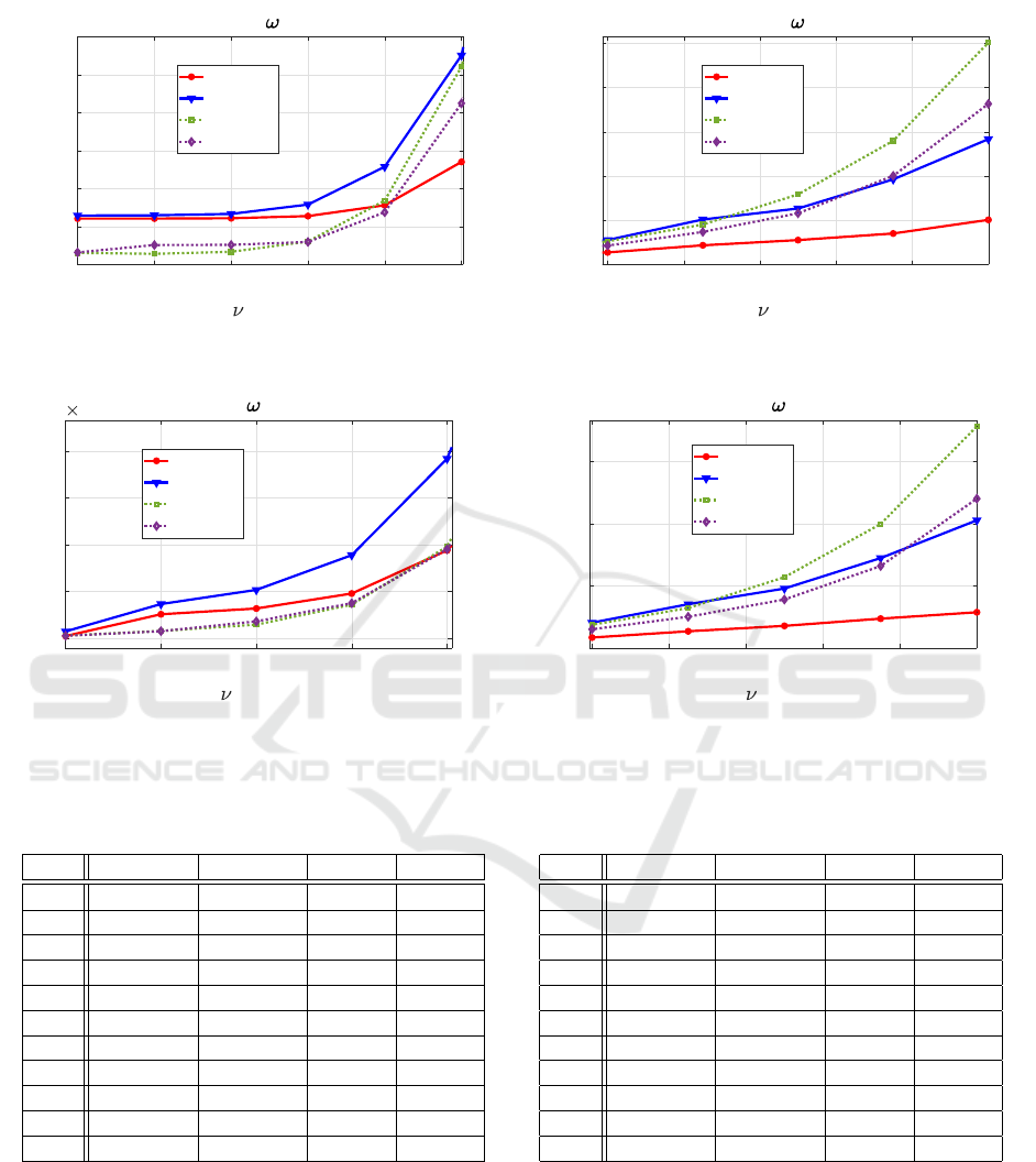
4.2 Results and Discussion
The values of RMSE for a fixed state noise bounds
and various observation noise are summarized in Ta-
ble 1 and visualised in Figure 1. The values of MAE
for a fixed state noise bounds and various observa-
tion noise are summarized in Table 2 and visualised in
Figure 2. Both criteria indicate that for lower noises,
LSUO and LSUP perform slightly better than both
LSUCZ variants. For higher noises, LSUCZ-1 out-
performs all other methods and LSUO is the worst
one.
ICINCO 2023 - 20th International Conference on Informatics in Control, Automation and Robotics
192

-3.5 -3 -2.5 -2 -1.5 -1
[log
10
]
0
0.005
0.01
0.015
0.02
0.025
RMSE, = 10
-4
LSUCZ 1
LSUCZ 2
LSUO
LSUP
-1 -0.8 -0.6 -0.4 -0.2 0
[log
10
]
0
0.05
0.1
0.15
0.2
0.25
RMSE, = 10
-4
LSUCZ 1
LSUCZ 2
LSUO
LSUP
Figure 1: RMSE of state estimates for ω = 10
−4
∗ 1
ℓ
x
and various ν, ν = 10
−K
∗ 1
ℓ
y
, K ∈ [0;4].
-4 -3.5 -3 -2.5 -2
[log
10
]
0
1
2
3
4
10
-3
MAE, = 10
-4
LSUCZ 1
LSUCZ 2
LSUO
LSUP
-1 -0.8 -0.6 -0.4 -0.2 0
[log
10
]
0
0.05
0.1
0.15
MAE, = 10
-4
LSUCZ 1
LSUCZ 2
LSUO
LSUP
Figure 2: MAE of state estimates for ω = 10
−4
∗ 1
ℓ
x
and various ν, ν = 10
−K
∗ 1
ℓ
y
, K ∈ [0;4].
Table 1: RMSE∗10
−3
of state estimates for state noise
bounds ω = 10
−4
∗ 1
ℓ
x
and various output noise bounds
ν = 10
−K
∗ 1
ℓ
y
.
K LSUCZ-1 LSUCZ-2 LSUO LSUP
4 < 10
−3
< 10
−3
< 10
−3
< 10
−3
3.5 6.0 6.4 1.5 1.6
3 6.0 6.5 1.4 2.5
2.5 6.1 6.6 1.6 2.6
2 6.4 7.9 3.0 2.9
1.5 7.8 12.9 8.4 6.9
1 13.5 27.5 26.1 21.2
0.75 21.5 50.7 45.1 36.7
0.5 27.4 63.2 79.1 57.8
0.25 34.9 96.1 139.8 100.1
0 50.3 141.7 250.8 181.5
The values of STD for a fixed state noise bounds
and various observation noise are visualised in Figure
3. While for lower noises, the results are compara-
ble for all filters, for the highest state noise, the both
LSUCZ variants perform better.
Table 2: MAE∗10
−3
of state estimates for state noise
bounds ω = 10
−4
∗ 1
ℓ
x
and various output noise bounds
ν = 10
−K
∗ 1
ℓ
y
.
K LSUCZ-1 LSUCZ-2 LSUO LSUP
4 < 10
−3
< 10
−3
< 10
−3
< 10
−3
3.5 0.5 0.7 0.1 0.1
3 0.6 1.0 0.3 0.4
2.5 0.9 1.8 0.7 0.7
2 1.9 3.8 2.0 1.9
1.5 3.9 8.8 5.9 4.8
1 8.4 20.4 18.7 15.0
0.75 13.4 35.2 32.2 25.1
0.5 17.8 47.8 56.9 39.0
0.25 23.6 72.2 99.6 65.9
0 28.7 102.6 178.0 120.0
5 CONCLUSION
This preliminary research suggests that constrained
zonotopes are a promising class to deal with a con-
strained uncertainty in the context of a Bayesian state
estimation. The proposed LSUCZ filter is more flex-
Bayesian State Estimation Using Constrained Zonotopes
193

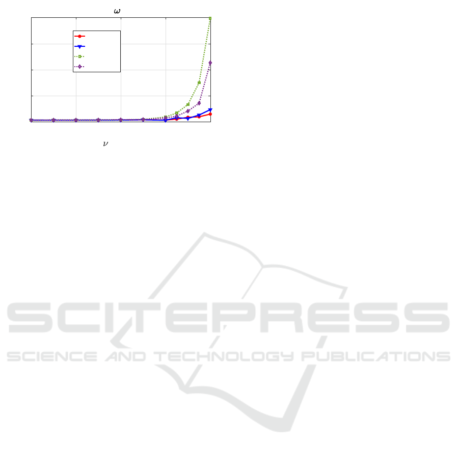
-4 -3 -2 -1 0
[log
10
]
0.48
0.5
0.52
0.54
0.56
STD, = 10
-4
LSUCZ 1
LSUCZ 2
LSUO
LSUP
Figure 3: STD of state estimates for ω = 10
−4
∗ 1
ℓ
x
and
various ν, ν = 10
−K
∗ 1
ℓ
y
, K ∈ [0;4].
ible compared to the previous LSUO and LSUP vari-
ants. It outperforms them from the point of view esti-
mation errors for higher observation noises.
The further research will focus on the more
detailed analysis including the posterior vol-
umes and using the the proposed LSUCZ fil-
ter in the task of a Bayesian transfer learning
schema (Kukli
ˇ
sov
´
a Pavelkov
´
a et al., 2022).
ACKNOWLEDGEMENTS
This research has been supported by GA
ˇ
CR grant 23-
04676J.
REFERENCES
Althoff, M. and Rath, J. J. (2021). Comparison of guaran-
teed state estimators for linear time-invariant systems.
Automatica, 130:109662.
Combastel, C. (2015). Zonotopes and Kalman observers:
Gain optimality under distinct uncertainty paradigms
and robust convergence. Automatica, 55:265 – 273.
Combastel, C. (2016). An extended zonotopic and Gaussian
Kalman filter merging set-membership and stochastic
paradigms: Toward non-linear filtering and fault de-
tection. Annual Reviews in Control, 42:232–243.
Ge, X., Han, Q., and Wang, Z. (2019). A dynamic
event-triggered transmission scheme for distributed
set-membership estimation over wireless sensor net-
works. IEEE Transactions on Cybernetics, 49(1):171–
183.
Jirsa, L., Pavelkov
´
a, L. K., and Quinn, A. (2019). Bayesian
filtering for states uniformly distributed on a parallelo-
topic support. In 2019 IEEE International Symposium
on Signal Processing and Information Technology (IS-
SPIT), pages 1–6. IEEE.
K
´
arn
´
y, M., B
¨
ohm, J., Guy, T. V., Jirsa, L., Nagy, I., Ne-
doma, P., and Tesa
ˇ
r, L. (2006). Optimized Bayesian
Dynamic Advising: Theory and Algorithms. Springer,
London.
Kotz, S. and Dorp, J. R. (2004). Beyond beta: Other con-
tinuous families of distributions with bounded support
and applications. World Scientific.
Kukli
ˇ
sov
´
a Pavelkov
´
a, L., Jirsa, L., and Quinn, A. (2022).
Fully probabilistic design for knowledge fusion be-
tween Bayesian filters under uniform disturbances.
Knowledge based systems, 238:107879.
Pan, Z., Luan, X., and Liu, F. (2022). Set-membership state
and parameter estimation for discrete time-varying
systems based on the constrained zonotope. Interna-
tional journal of control.
Pavelkov
´
a, L. and Jirsa, L. (2018). Approximate recursive
Bayesian estimation of state space model with uni-
form noise. In Proceedings of the 15th ICINCO con-
ference, pages 388–394.
Raghuraman, V. and Koeln, J. P. (2022). Set operations and
order reductions for constrained zonotopes. Automat-
ica, 139:110204.
Rego, B. S., Raffo, G. V., Scott, J. K., and Raimondo, D. M.
(2020a). Guaranteed methods based on constrained
zonotopes for set-valued state estimation of nonlinear
discrete-time systems. Automatica, 111:108614.
Rego, B. S., Raimondo, D. M., and Raffo, V, G. (2020b).
Set-based state estimation and fault diagnosis of lin-
ear discrete-time descriptor systems using constrained
zonotopes. IFAC PapersOnLine, 53(2):4291–4296.
Samada, S. E., Puig, V., and Nejjari, F. (2023). Zonotopic
recursive least-squares parameter estimation: Appli-
cation to fault detection. International Journal of
Adaptive Control and Signal Processing, 37(4):993 –
1014.
S
¨
arkk
¨
a, S. (2013). Bayesian Filtering and Smoothing. Cam-
bridge University Press.
Scott, J. K., Raimondo, D. M., Marseglia, G. R., and Braatz,
R. D. (2016). Constrained zonotopes: A new tool for
set-based estimation and fault detection. Automatica,
69:126–136.
Shao, X., Huang, B., and Lee, J. M. (2010). Constrained
Bayesian state estimation–a comparative study and a
new particle filter based approach. Journal of Process
Control, 20(2):143–157.
Sharma, U., Thangavel, S., Mukkula, A. R. G., and Paulen,
R. (2018). Effective recursive parallelotopic bounding
for robust output-feedback control. IFAC Paperson-
line, 51(15):1032–1037.
Simon, D. and Simon, D. L. (2010). Constrained Kalman
filtering via density function truncation for turbofan
engine health estimation. International Journal of
Systems Science, 41:159–171.
ICINCO 2023 - 20th International Conference on Informatics in Control, Automation and Robotics
194