Multiple Additive Neural Networks: A Novel Approach to Continuous

Learning in Regression and Classiﬁcation

Janis Mohr

, Basile Tousside

, Marco Schmidt

and J

org Frochte

Interdisciplinary Institute for Applied Artiﬁcial Intelligence and Data Science Ruhr, Bochum University of Applied

Sciences, 42579 Heiligenhaus, Germany

Keywords:

Gradient Boosting, Machine Learning, Continuous Learning, Neural Networks, Overﬁtting.

Abstract:

Gradient Boosting is one of the leading techniques for the regression and classiﬁcation of structured data.

Recent adaptations and implementations use decision trees as base learners. In this work, a new method based

on the original approach of Gradient Boosting was adapted to nearly shallow neural networks as base learners.

The proposed method supports a new architecture-based approach for continuous learning and utilises strong

heuristics against overﬁtting. Therefore, the method that we call Multiple Additive Neural Networks (MANN)

is robust and achieves high accuracy. As shown by our experiments, MANN obtains more accurate predictions

on well-known datasets than Extreme Gradient Boosting (XGB), while also being less prone to overﬁtting and

less dependent on the selection of the hyperparameters learn rate and iterations.

1 INTRODUCTION

Boosting is a technique that combines weak learn-

ers to achieve a highly accurate model. Every sin-

gle learner only needs to be moderately accurate

(Shapire, 1990).

Gradient Boosting is a proposed boosting tech-

nique that has had great success on data sets with

structured data (Friedman, 1999b; Viola and Jones,

2001). Most published papers use different imple-

mentations of decision trees as base learners (Chen

and Guestrin, 2016; Dorogush et al., 2018). The

gradient of a previous learner is used for ﬁtting the

next learner in Gradient Boosting. Gradient Boost-

ing can achieve very accurate predictors and is less

prone to overﬁtting than other boosting techniques,

but still easily overﬁts on some datasets if several

hundred learners are combined (Bikmukhametov and

Jaeschke, 2019). The MANN algorithm is an adap-

tation and enhancement of the gradient boosting al-

gorithm with nearly shallow neural networks as base

learners. Several heuristics and techniques are used

to prevent overﬁtting. Thus, MANN can reach better

accuracy than popular implementations of Gradient

https://orcid.org/0000-0001-6450-074X

https://orcid.org/0000-0002-9332-5060

https://orcid.org/0000-0002-7232-5256

https://orcid.org/0000-0002-5908-5649

Boosting which are based on weak learners like de-

cision trees. We especially emphasise developing an

algorithm that is easy to use and supports continuous

learning rather than being mainly focused on accu-

racy. Our approach focuses on using neural networks

with a minimum of hidden layers and neurons. We

present techniques to automatically stop the training

of new neural networks if accuracy is not signiﬁcantly

improved.

Some papers have already considered the possi-

bility of using boosting techniques with neural net-

works. (Schwenk and Bengio, 2000) used neural

networks in combination with the Adaptive Boosting

(AdaBoost) method and came to the conclusion that

it works as well and sometimes even better than Ad-

aBoost with decision trees. Our experiments rely on

the newer, more general, and (in effective implemen-

tations) better-performing Gradient Boosting. The re-

sults conﬁrm the good quality of predictions of boost-

ing with neural networks. Additionally, advanced

heuristics were added and the algorithm was designed

to be easy to use and reduce hyperparameter tuning.

(Martinez-Munoz, 2019) proposes to train the

neurons of a single neural network with one hidden

layer sequentially in a boosting approach. (Shalev-

Shwartz, 2014) proposed the SelﬁeBoost algorithm

that uses Stochastic Gradient Descent as a weak

learner for boosting a single neural network.

A recently followed path of research is the com-

540

Mohr, J., Tousside, B., Schmidt, M. and Frochte, J.

Multiple Additive Neural Networks: A Novel Approach to Continuous Learning in Regression and Classiﬁcation.

DOI: 10.5220/0012234000003595

In Proceedings of the 15th International Joint Conference on Computational Intelligence (IJCCI 2023), pages 540-547

ISBN: 978-989-758-674-3; ISSN: 2184-3236

bination of trees and neural networks. Papers in this

domain use tree-like structures with neural networks.

Adaptive Neural Trees (Tanno et al., 2018) adaptively

grow tree-like structures with neural networks. (De-

boleena et al., 2018) proposes to build a hierarchical

model out of several neural networks in a tree-wise

manner which can grow to learn new data. MANN

differs from these approaches because it is based on

an algorithm commonly used with decision trees but

does not try to put neural networks into tree-like struc-

tures.

This paper will enhance the related work regard-

ing overﬁtting and adaptivity, showing how to use

Gradient Boosting with neural networks and that it

achieves even better predictions than popular boost-

ing algorithms. Our approach to achieving highly ac-

curate predictors was extended with continuous learn-

ing, which furthermore separates our algorithm from

plain implementations of Gradient Boosting. Several

real-life use-cases of machine learning beneﬁt from

continuous learning (Kaeding et al., 2017). New data

is generated over time and while an already trained

model is in use. MANN is eminently suitable in

these cases to continuously train a model and im-

prove its accuracy on new data. Our algorithm al-

lows two different approaches to support continuous

learning, altering the neural networks of an already

existing model and calculating residuals with the al-

ready trained model to ﬁt a new model and create a

combined model. Special attention was given to over-

ﬁtting as a general problem in machine learning. An

implementation of a heuristic that works to prevent

overﬁtting when using Gradient Boosting with neural

networks is proposed and it is shown that MANN is

less prone to overﬁtting and easier to use because of

less hyper-parameter tuning than other popular boost-

ing techniques.

Our speciﬁc contributions in this paper are sum-

marised below:

1. We propose a novel method that incrementally

builds deep neural networks out of several neural

networks using the Gradient Boosting algorithm.

This method is versatile and can easily be adapted

for a wide range of tasks and domains while being

easier to train and ﬁne-tune than traditional deep

neural networks.

2. We develop heuristics against overﬁtting based on

early stopping for this method and propose an

architecture-based approach for continuous learn-

ing.

3. We demonstrate the usefulness of the developed

heuristics and the approach for continuous learn-

ing. Furthermore, we show superior results on

several regression and classiﬁcation datasets.

2 AN APPROACH FOR ADDITIVE

NEURAL NETWORKS

The accuracy of a predictive model can often be in-

creased by averaging the decisions of an ensemble of

predicitve models. When the individual predictors are

accurate and diverse, signiﬁcant improvement can be

expected. A general idea to use this is to have a base

learner and apply it on different training sets for sev-

eral times.

Gradient Boosting is a boosting algorithm. It se-

quentially trains predictors to construct an additive

model. The gradient of the loss function is used to

train the predictor on the next iteration. All ﬁtted pre-

dictors have the same inﬂuence on the ﬁnal model,

only weighted by a learning rate that is equal for all

predictors. Gradient Boosting as proposed by (Fried-

man, 1999a) is a two-step optimisation method.

A system of output (target) variables y and input

variables (features) x can be formed into a dataset

D = {y

, x

}. The goal for our algorithm is then to

model a function F

∗

(x) on the dataset D of known

(y, x)-values. The function F

∗

(x) maps x to y in a

way that the value of a speciﬁed differentiable loss

function L(y

, F(x)) is minimised. The index j is the

ongoing number of the iteration I

The algorithm starts with an initial guess F

(x),

which is a constant value. This initial guess is used

as a starting point for the model. At this point, the

model would predict F

(x) for every value of x. In the

second step, the (pseudo-)residuals are computed as:

i, j

= −[

∂L(y

, F(x

))

∂F(x

)

]

F(x)=F

j−1

(x)

(1)

The term (pseudo-)residuals is used because their na-

ture depends on the loss function. For example the

loss function residual sum of squares L(y

, F(x)) =

· (y

− F(x))

which is mostly used for regression

leads to real residuals (Friedman, 1999a). The base

learner is then ﬁt to the (r

, x

)-values. Next, the out-

put values γ

of the ﬁtted base learner for the whole

dataset are computed with γ being the predicted value

for the current residuum.

= argmin

∑

∈R

i, j

L(y

, F

j−1

) + γ) (2)

Finally, the predictions F

(x) of the model at the cur-

rent iteration I

are computed. The predictions of the

previous iteration are summed up with the predictions

of the current iteration and are multiplied by a learn-

ing rate ν as proposed by (Friedman, 1999a). The

learn rate assures that every base learner’s inﬂuence

in the ﬁnal model is limited. This limitation reduces

Multiple Additive Neural Networks: A Novel Approach to Continuous Learning in Regression and Classiﬁcation

541

1: Input: data x

, y

; Loss function L(y

, F(x))

2: Initialise F

(x) = argmin

∑

i=1

L(y

, γ).

3: repeat

4: r

i, j

= −[

∂L(y

,F(x

))

∂F(x

)

]

F(x)=F

j−1

(x)

5: Fit a neural network to r

i, j

6: Early stopping.

7: for j = 1, ..., J

8: γ

= argmin

∑

∈R

i, j

L(y

, F

j−1

) + γ)

9: end for

10: F

(x) = F

j−1

(x) + ν

∑

j=1

11: Heuristic to prevent overﬁtting.

12: j = j + 1

13: until j = J

Algorithm 1: Multiple Additive Neural Networks.

the impact of a non-optimal iteration.

(x) = F

j−1

(x) + ν

∑

j=1

(3)

The process of computing the residuals, ﬁtting the

base learner, and updating the predictions is done se-

quentially for a given number of iterations J. After

reaching J iterations the model is considered com-

plete and trained. This trained model is called M and

is ready to be used for predictions.

This description of Gradient Boosting is abstract

and not restricted to one speciﬁc type of base learner

or loss function. Most implementations use decision

trees as base learners. MANN uses neural networks

as base learners. The networks can be used for re-

gression and classiﬁcation tasks. The main idea be-

hind using artiﬁcial neural networks is that Gradient

Boosting might be able to accomplish better accuracy

with stronger base learners while allowing continuous

learning by directly retraining the neural networks.

The established theory of gradient boosting is

used to present a new approach for neural networks

offering the previously described advantages. Not

quite so deep (no more than three hidden layers) neu-

ral networks are used and therefore gradient boosted

neural networks for both regression and classiﬁca-

tion are the core of MANN. The efﬁciency of neu-

ral networks depends on choosing reasonable hyper-

parameters for their structure and training. The arti-

ﬁcial neural networks are kept as small and shallow

as possible. The number of neurons on every layer

can be adapted. To predict complex functions, higher

numbers of neurons are necessary. On every itera-

tion I

in the algorithm, the (pseudo-)residuals are

calculated. A neural network NN

is ﬁtted on these

(pseudo-)residuals. The neural network then predicts

the original unaltered training dataset D. These pre-

dictions are used to calculate the (pseudo-)residuals

on which a neural network is ﬁtted in the next itera-

tion. The number of epochs that a single neural net-

work is trained in is automatically regulated with an

implementation of early stopping. The progress the

neural network makes on the training dataset is eval-

uated after every epoch. If the accuracy of the neural

network does not increase further for a given amount

of epochs the training is stopped prematurely.

2.1 Heuristic to Prevent Overﬁtting

1: Let T be the training set and V the validation set.

2: Every time training of a neural network NN

ﬁnished:

3: if E

(NN

) ≥ E

(NN

i−1

)or ≤ E

then

4: break

5: end if

Algorithm 2: Heuristic to prevent overﬁtting.

Preventing Overﬁtting is a central and important part

of every algorithm that ﬁts neural networks on data.

Our heuristic takes action after operation 10 on

line 10 in algorithm 1. The heuristic is used on ev-

ery iteration of our algorithm. An amount of data is

removed from the training dataset T and used as the

validation dataset V . The validation dataset remains

unaltered during the algorithm and is used on every

iteration. Tests on several datasets have shown that

taking ﬁve percent of the test data as validation data

delivers good results. Algorithm 2 shows the used

heuristics schematically.

On the current iteration I a model M

is built up

out of the initial value F

and the already ﬁtted neural

networks NN

. This temporary model represents the

current state of the training and how the model would

perform if the ﬁtting of new neural networks would

be stopped now.

is now fed with the x values of the validation

dataset to make predictions on it. The predictions are

evaluated and an error E

is calculated. This error is

compared to a threshold E

. If it is below this thresh-

old the model predicts as well as wanted and the ﬁt-

ting of new neural networks is stopped. Otherwise,

the training continues. Over n steps the accuracy of

predictions is evaluated. If the accuracy is steady or

decreases, the ﬁtting of additional neural networks is

also stopped because no improvements are to be ex-

pected. During experiments, it seemed reasonable to

choose n = 3.

Our heuristics securely prevent overﬁtting and fur-

thermore reduce the time needed for computation.

The ﬁtting of additional neural networks is stopped

when no improvement is to be expected. Therefore,

NCTA 2023 - 15th International Conference on Neural Computation Theory and Applications

542

the algorithm is user-friendly and easy to use. Over-

ﬁtting is automatically avoided without any parame-

ter tuning. Our algorithm also automatically avoids

waste of time and energy from ﬁtting neural networks

that do not improve the accuracy of the model further.

In the same mind, an early stopping (Raskutti

et al., 2013) was added on the level where the neural

networks are trained (algorithm 1 operation 5). For

every evaluation, the same evaluation dataset is used.

The performance of the single neural networks is con-

stantly evaluated every epoch. If no progress is made

for a number of steps the training of this neural net-

work is stopped because it is not expected to achieve

better performance.

The proposed algorithm prevents overﬁtting and

training without any positive effect on the perfor-

mance of the model on two levels. Every neural net-

work is accurately monitored and trained in the opti-

mal amount of epochs. Additionally, the whole model

is evaluated at every iteration to keep it as small as

possible and make it less prone to overﬁtting.

2.2 Architecture-Based Approach to

Continuous Learning

1: Let T

and T

be two datasets with the same num-

ber of features and the same target value.

2: Model M

trained on T

as described in Algo-

rithm 1.

3: if E(M

)) − E(M

)) ≥ ε then

4: break

5: else

6: Retrain Model M

on the new training data T

7: if |E(M

)) − E(M

))| ≥ ε then

8: break

9: else

10: Algorithm 1 with T

to build Model M

11: Combine M

and M

to create ﬁnal Model

12: end if

13: end if

Algorithm 3: Continuous Learning with MANN.

Humans have the ability to acquire and transfer

knowledge throughout their life. This is called life-

long learning. Continuous learning is an adaption of

this mechanic (Kaeding et al., 2017). In this paper,

continuous learning is considered to be a technique

that allows a complete model to be able to predict a

new dataset with the same features. Therefore, it must

be retrained or expanded. An algorithm that supports

both the time-efﬁcient retraining and the expansion

of the model was developed. This technique is only

suitable for continuous learning with a dataset with

the same classes as the original dataset otherwise it

would be necessary to alter at least the last layer of

the neural networks. The algorithm is not only supe-

rior in terms of accuracy as the experiments show but

it also supports continuous learning on two levels.

A model M

is trained on a dataset T

. This model

reaches a certain quality of its predictions until the

training is stopped. A second dataset T

exists with

new data but the same set of features and targets as the

ﬁrst dataset. For example, this could be data that was

gathered after the training on the original data was

ﬁnished. It would be possible to train a new model

on a dataset constructed out of both datasets. But it is

much more feasible to use the already ﬁtted model to

reduce the amount of time needed for training a new

model from scratch, especially on very large datasets.

It will require some retraining.

First, the algorithm checks if new training is re-

quired. The already trained model is fed with the new

data and the predictions of the model are evaluated

by comparing the error E of the prediction of T

with

the error E of the prediction of T

. If the results in a

speciﬁc metric are close to the original dataset, appar-

ently retraining is not necessary. It is very likely that

better results will not be achieved. The two datasets

seem to be quite similar.

|E(M

)) − E(M

))| ≥ ε (4)

Given the case that there is a difference in the

accuracy of predictions, the new dataset is used for

training. At ﬁrst, the already existing neural networks

in the model are retrained on the new dataset. There-

fore, the weights are adapted to ﬁt the new data bet-

ter. After this assimilation, the new dataset is again

predicted with the model. If the performance is simi-

lar to the original one there is no need to continue the

training. Equation (4) is again used for the rating of

the performance. E can be an arbitrary error metric

for example mean-square-error. If there is still a sig-

niﬁcant difference the model is extended. Algorithm

1 is used again but with the new dataset. Generally

speaking, new neural networks that are ﬁtted to the

new dataset are added to the already existing model

The algorithm starts off with the initial guess

(x). When not training continuously the target val-

ues y

are used for initialisation. Taking advantage

of already having a model, the loss of Model M

training data T

is used as the initial value. There-

fore, model M

is used to start the ﬁtting of new neu-

ral networks. From this point on, model M

is built

with neural networks that are ﬁt to the data for a given

amount of iterations I. The ﬁnal model is M

and is

then used for predictions. Continuous learning can be

repeated as new training data becomes available. This

Multiple Additive Neural Networks: A Novel Approach to Continuous Learning in Regression and Classiﬁcation

543

approach to continuous learning is especially suitable

for regression tasks. The complete process of contin-

uous learning as pseudo-code is given in Algorithm

3 EXPERIMENTS

In the following section, different experiments are de-

scribed. The experiments show the accuracy of the

proposed method and how it works including demon-

strations of the effectiveness of the heuristics against

overﬁtting. An academic implementation of MANN

is used for the experiments. The loss function

L(y

, F(x)) =

· (y

− F(x))

is used for regression

tasks and the loss function L(y

, p) = y

· log(p) +

(1 − y

) · log(1 − p), with the predicted probability

p, is used for classiﬁcation. The implemented arti-

ﬁcial neural networks have three hidden layers with

8 neurons each. We decided to use this ﬁxed set of

layers and neurons to reduce the variation of parame-

ters during the following experiments. This strongly

enhances the validity of the experiments and aligns

the number of hyperparameters that are available

throughout the compared learners. Extensive repeti-

tions of the experiments were done to ensure that the

parameters are chosen in a way that the neural net-

works achieve good performance. XGB is used to

compare and evaluate the performance. The freely

available implementation of XGB was used. In the re-

gression experiments, a multi-layer perceptron (MLP)

with 5 layers was used as an example of the perfor-

mance of deep neural networks without any boosting.

3.1 Results on Regression Benchmarks

The following sections contain a study on the perfor-

mance on several regression benchmarks to show off

the accuracy of MANN compared to other popular

methods.

3.1.1 Results on the Bike Sharing Dataset

In this experiment, a dataset known as the Bike Shar-

ing dataset is used. It is a popular dataset that was re-

leased in 2013 and since then used to test algorithms

and for educational purposes (Fanaee-T and Gama,

2014).

Data for every rented bike is logged. The informa-

tion consists out of duration, start date, end date, start

station, end station, bike number, and member type.

This data is enhanced with general information about

the environment like weather, humidity, temperature,

wind speed, and weekday. The dataset has data for

every hour for two years which leads to 17,379 rows

of data. Each with 15 features.

First, training is started on the whole dataset. Data

augmentation or elimination of outliers was not done.

The unaltered dataset is used for our experiment to

have a good comparison to the accuracy of XGB on

the same dataset. A parameter grid search was used

to ﬁnd the best combination of learn rate and itera-

tions with a maximum of 500 epochs. Stochastic gra-

dient descent was used as optimiser and the ﬁtting

of new networks was halted when the mean-absolute

error on the validation dataset falls below 1. The

learning rate was set to 0.3. With these parameters,

an RMSE of 56 was achieved in predicting the test

data. The data from the last days of every month,

starting with the 20th was used as test data to have

a use case that is close to real life. For comparison,

a XGB model is trained on the same dataset with a

learning rate of 0.2 and a maximum tree depth of 6.

This XGB model acquired an RMSE of 62 on the test

data. These results lead to two insights. Firstly XGB

overﬁts the dataset with reasonably picked parameters

while MANN does not. Secondly, the accuracy of the

prediction is better with MANN.

The aforementioned parameters for both methods

were chosen with a parameter grid search and are the

parameters that had the best results. Figure 1 is a

plot of the RMSE over the iterations and learn rate

for MANN and XGB.

MANN has a peak for a combination of a small

learn rate and few iterations. This suggests avoiding

choosing small learn rates and few iterations, which

is consistent. XGB shows overﬁtting on this dataset

strongly depending on the learn rate. With a higher

learn rate the overﬁtting increases. This experiment

demonstrates that the heuristic proposed in section

2.1 is working. To furthermore prove the claim that

the proposed heuristics work, MANN was used to

train a model on the bike-sharing dataset with and

without the heuristic. The accuracy on the training

data increases progressively for the model without the

heuristics and decreases on the test data. The other

model keeps improving until no more improvement

can be made and then stops.

3.1.2 Million Song Dataset & CT Scan Slize

Localization Dataset

The CT Scan Slize Localization Dataset is a dataset

with medicinal data proposed by (Graf et al., 2011). It

consists of 384 features extracted from a set of 53500

CT images from 74 different patients (43 male, 31 fe-

male). The ﬁnal feature vector is a concatenation of

two histograms, one about the location of bone struc-

tures and one about air inclusions. The target values

NCTA 2023 - 15th International Conference on Neural Computation Theory and Applications

544

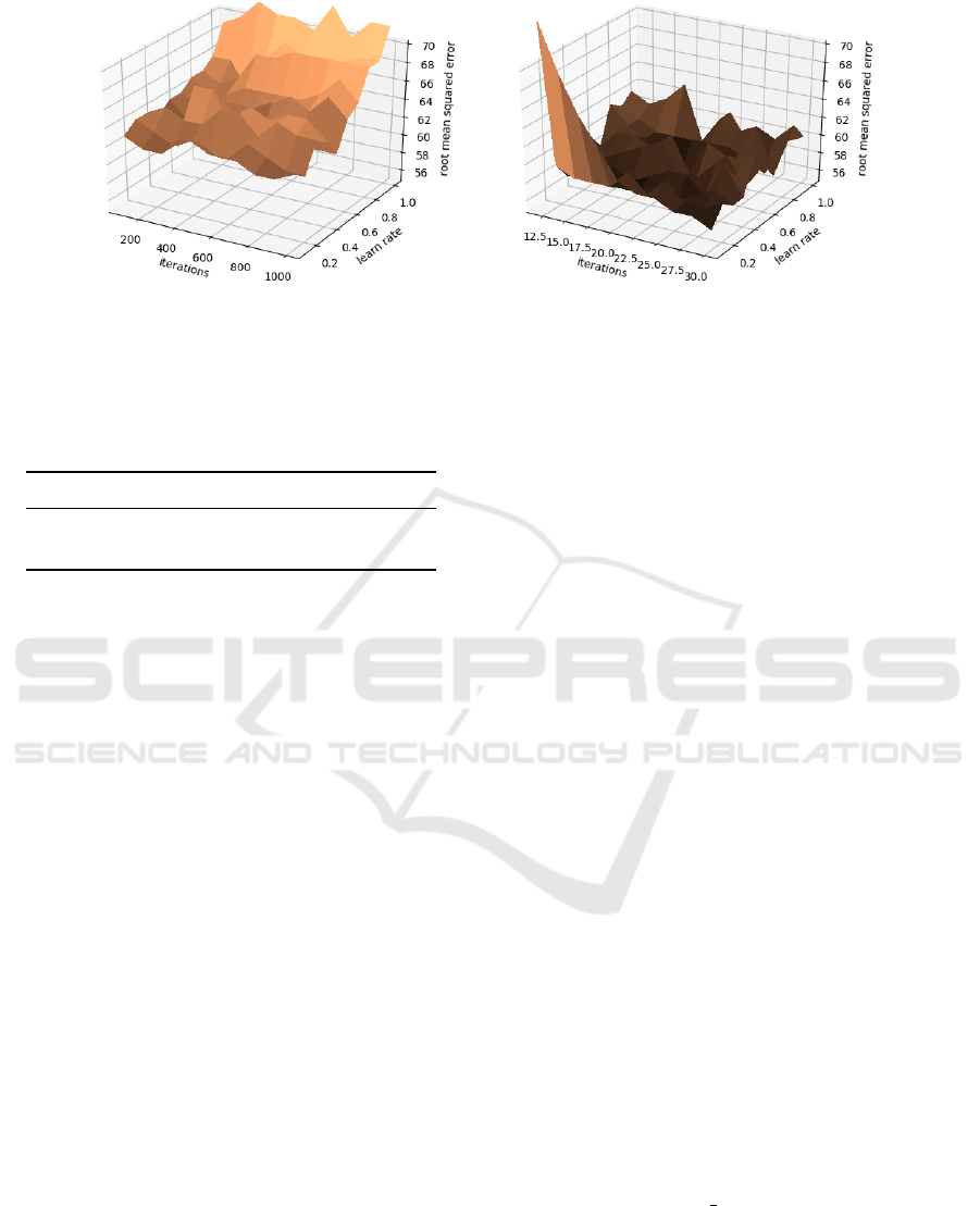
Figure 1: RMSE plotted depending on the number of iterations and learn rate training the bike sharing dataset with XGB (left)

and MANN (right). This plot represents the parameter grid search that was used to ﬁnd the parameters for MANN and XGB

that lead to the best accuracy. The root mean squared error is used as a metric. Furthermore, this plot shows that MANN is

less dependent on its parameters then XGB.

Table 1: Regression Datasets (CT Scan and MSD in

RMSE).

Dataset MANN XGB ANT MLP

CT Scan 5.34 6.67 - 8.49

MSD 8.57 9.38 - 12.73

are in a range from 0 to 180.

The Million Song Dataset (MSD) is a set of fea-

tures for songs from 1922 to 2011 published by

(Bertin-Mahieux et al., 2011). Predicting a track’s

year of origin based only on audio features and with-

out any metadata is the task. The split into test

and training data recommended by the authors of the

dataset is used to avoid having artists appear in both

training and test data. The data per year is highly non-

uniformly distributed. All results can be seen in table

3.2 Results on Binary Classiﬁcation

Datasets

As described in Section 2 MANN does not only sup-

port regression but also classiﬁcation tasks. Three bi-

nary classiﬁcation datasets were selected to present a

variety of complexity and dataset sizes and the accu-

racy of MANN, XGB, and ANT are compared. Re-

sults can be seen in table 2.

3.2.1 UCI Heart Disease & Rain in Australia

Dataset

The UCI heart disease dataset was published by (De-

trano et al., 1989). This dataset consists out of 4

subsets from different hospitals with data on patients

with and without heart disease. The goal is to predict

whether a patient has heart disease and if so, which

type. It has 14 features and 303 instances that rep-

resent medical data about patients and it reduces the

task to ﬁnd out if a patient has heart disease or not.

While some papers (Dangare and Apte, 2012;

Zriqat et al., 2016) reach an accuracy of nearly 100

percent on this dataset with the use of heavy data

augmentation most papers (Chen et al., 2011; Sabar-

inathan and Sugumaran, 2014; Sabay et al., 2018)

reach an accuracy of around 85 percent without any

data augmentation. No data augmentation was used

in this experiment for better comparability.

A learning rate of 0.6 and 18 neural networks were

used. Every neural network was trained in a maxi-

mum of 400 epochs.

With these parameters, MANN reaches an accu-

racy of 90 percent and XGB of 85 percent. MANN is

more accurate than XGB and is also slightly above

what most published papers (Aljanabi et al., 2018)

accomplish on this dataset showing that MANN

works well on very small datasets.

The rain in Australia dataset contains daily

weather information from different locations all over

Australia. The target is to predict whether it is go-

ing to rain the next day. The dataset consists of 23

features in 142,193 rows. Data was collected from

different weather stations in Australia over a time of

10 years. The data origins from the Bureau of Meteo-

rology of the Australian government. Predicting rain-

fall is of immense interest because it can be an early

warning sign for natural disasters and is important for

agriculture (Parmar et al., 2017).

The feature RISK MM was excluded from the

training dataset. It is the amount of rainfall that oc-

curred on the next day and was used as a source to

ascertain the value for the target variable. Several fea-

tures are categorical, for example, the wind direction.

Label Encoding was used to deal with all categorical

Multiple Additive Neural Networks: A Novel Approach to Continuous Learning in Regression and Classiﬁcation

545

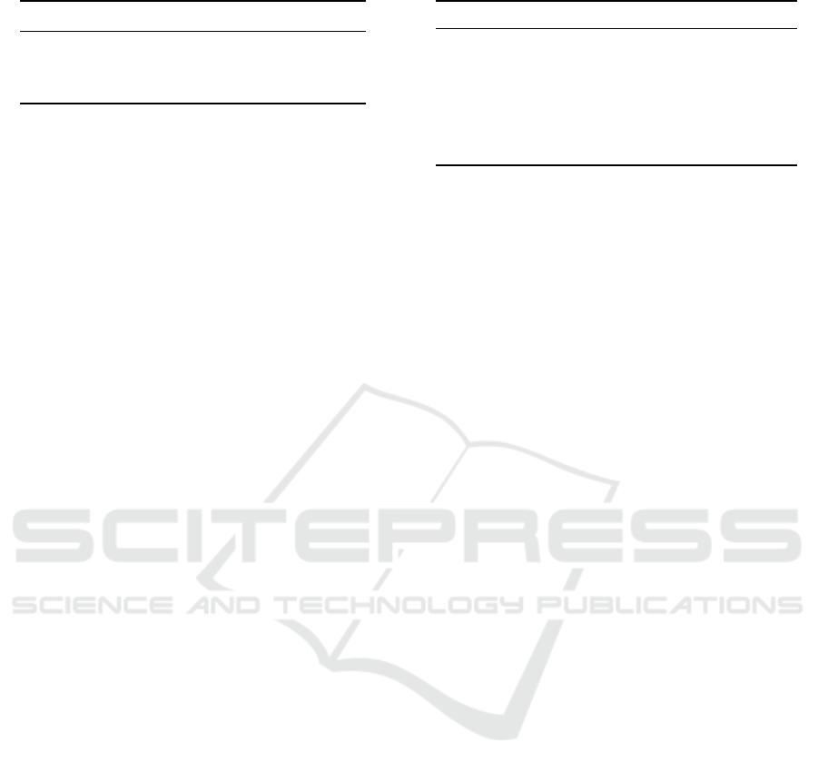
Table 2: Binary Classiﬁcation Datasets Accuracy.

Dataset MANN XGB ANT

UCI heart disease 0.90 0.85 0.88

Rain in Australia 0.89 0.87 0.89

Higgs Boson 0.85 0.83 0.82

features present in the Rain in Australia dataset.

The best results were found with a parameter grid

search with a learn rate M

= {ν ∈ N|2 ≤ ν ≤ 20∧ν =

2 × k} for both learners. 600 iterations were used for

XGB and 18 for MANN. The development of the ac-

curacy is steady for XGB with one peak and a mean of

85.04 percent accuracy. The best accuracy for XGB is

87 percent with a learn rate of 0.4 and 600 iterations.

MANN reaches a better accuracy of 89 percent with a

learn rate of 0.5 and 18 iterations. It has a mean accu-

racy of 84.87 percent. With an accuracy of 89 percent

ANT is as good as MANN on this task.

3.2.2 Higgs Boson Dataset

The Higgs Boson dataset is a classiﬁcation problem

to distinguish between a signal process that produces

Higgs bosons and a process that does not produce

Higgs Bosons. Monte Carlo simulations were used to

create the data. The features in this dataset represent

kinematic properties and some derived functions, usu-

ally used by physicists. The full dataset consists out of

1 million entries. (Baldi et al., 2014) This dataset was

used to evaluate the accuracy of MANN on a big and

imbalanced (there are many more data for not produc-

ing a Higgs boson) dataset. Again results can be seen

in table 2.

3.3 Continuous Learning Benchmark

The Bike Sharing dataset will be revisited to demon-

strate the strength of our continuous learning. The

dataset was divided into two independent pieces of

similar size and with the same features because the

data’s structure already clearly indicates to do so. The

split is done into two years 2011 and 2012. On av-

erage the number of rented bikes in 2012 is higher

than in 2011. A model M

was trained with MANN

with the same parameters mentioned above on the

ﬁrst part of the dataset. The model predicts the 2011

dataset with a root-mean-squared error of 57. Pre-

dicting the 2012 dataset with this model though leads

to a root-mean-squared error of 128. The already

trained model is used and continuously ﬁt on the sec-

ond dataset that relates to the log of 2012 in the man-

ner that is explained in section 2.2. The neural net-

works from model M

are retrained with the new data.

The RMSE improves to 106 and therefore the second

Table 3: Bike Sharing Comparison RMSE.

ALGORITHM 2011 2012 BOTH

MANN FROZEN 57 128 56

MANN CL 1ST LEVEL 57 106 56

MANN CL ALL LEVELS 57 79 56

XGB FROZEN 58 130 62

LEARN++.MT 60 87 63

ANN FROZEN 69 155 67

ANN CL 69 92 67

level of continuous learning takes effect. Neural net-

works are trained on the new data and then added to

the already existing model. An RMSE of 79 is the re-

sult of the new model combining both levels of con-

tinuous learning. The neural networks of the orig-

inal model were modiﬁed and new neural networks

trained on the 2012 dataset were added. XGB trained

on the 2011 dataset achieves a root-mean-squared er-

ror of 58. Trained on the 2011 dataset it reaches

an RMSE of 130 on the 2012 dataset. An artiﬁcial

neural network with 5 hidden layers and 20, 15, 10,

5, and 1 neurons trained in 700 epochs achieves an

RMSE of 69 and 155. This ANN was retrained on the

2012 dataset. After retraining, the RMSE on the 2012

dataset is 92. Learn++.MT, an algorithm that is based

on AdaBoost with decision trees and speciﬁcally pro-

posed for incremental learning by (Muhlbaier et al.,

2004) was also tested. All results can be seen in table

4 CONCLUSION

This paper proposed a novel approach for regression

and classiﬁcation machine learning tasks based on

the well-known and highly popular Gradient Boost-

ing framework. The original Gradient Boosting al-

gorithm was altered to use artiﬁcial neural networks

as base learners. MANN makes heavy use of early

stopping and a heuristic to prevent overﬁtting. Both

make our algorithm effective and easy to use with

a minimum of hyper-parameter tuning. We demon-

strated that our algorithm achieves better results on

datasets than popular implementations of the Gradient

Boosting algorithm for example XGB. Our algorithm

makes signiﬁcant improvements in prediction accu-

racy. Our algorithm also has a built-in method for

continuous learning. MANN can change the weights

of neural networks in an already trained model or train

new neural networks on a new dataset and add them

to an already trained model. It is sensible to do more

experiments with continuous learning and try to over-

come catastrophic forgetting with even the most elab-

orate learning tasks. Furthermore, it makes sense to

NCTA 2023 - 15th International Conference on Neural Computation Theory and Applications

546

look into possibilities to not only add more models or

retrain existing models but also to ﬁne-tune the exist-

ing neural networks or maybe even speciﬁc layers to

use this algorithm in incremental learning tasks. In

future research, it would make sense to add support

for unstructured data.

ACKNOWLEDGEMENTS

This work was funded by the Federal Ministry of Ed-

ucation and Research under 16-DHB-4021.

REFERENCES

Aljanabi, M., Qutqut, M. H., and Hijjawi, M. (2018). Ma-

chine learning classiﬁcation techniques for heart dis-

ease prediction: A review. International Journal of

Enigneering and Technology.

Baldi, P., Sadowski, P., and Whiteson, D. (2014). Searching

for exotic particles in high-energy physics with deep

learning. Nature Communications.

Bertin-Mahieux, T., Ellis, D. P., Whitman, B., and Lamere,

P. (2011). The million song dataset. In Proceedings of

the 12th International Conference on Music Informa-

tion Retrieval (ISMIR 2011).

Bikmukhametov, T. and Jaeschke, J. (2019). Oil production

monitoring using gradient boosting machine learning

algorithm. 12th IFAC Symposium on Dynamics and

Control of Process Systems.

Chen, A. S., Huang, S.-W., Hong, P. S., Cheng, C., and Lin,

E. J. (2011). Hdps: Heart disease predictions system.

Computing in Cardiology.

Chen, T. and Guestrin, C. (2016). Xgboost: A scalable tree

boosting system. KDD 16.

Dangare, C. S. and Apte, S. S. (2012). A data mining ap-

proach for predictions of heart disease using neural

networks. International Journal of Computer Engi-

neering and Technology, pages 30–40.

Deboleena, R., Priyadarshini, P., and Kaushik, R. (2018).

Tree-cnn: A hierarchical deep convolutional neural

network for incremental learning.

Detrano, R., Janosi, A., Steinbrunn, W., Pﬁsterer, M.,

Schmid, J.-J., Sandhu, S., Kern H. Guppy, S. L., and

Froehlicher, V. (1989). International application of a

new probability algorithm for the diagnosis of coro-

nary artery diseas. The American Journal of Cardiol-

ogy.

Dorogush, A. V., Ershov, V., and Gulin, A. (2018). Cat-

boost: gradient boosting with categorical features sup-

port. Conference on Neural Information Processing

Systems (NeurIPS 2018).

Fanaee-T, H. and Gama, J. (2014). Event labeling combin-

ing ensemble detectors and background knowledge.

Progress in Artiﬁcial Intelligence, pages 113–127.

Friedman, J. H. (1999a). Greedy function approximation: A

gradient boosting machine. The Annals of Statistics.

Friedman, J. H. (1999b). Stochastic gradient boosting.

Computational Statistics & Data Analysis, 38.

Graf, F., Kriegel, H.-P., Schubert, M., P

olsterl, S., and Cav-

allaro, A. (2011). 2d image registration in ct images

using radial image descriptors. In Fichtinger, G., Mar-

tel, A., and Peters, T., editors, Medical Image Com-

puting and Computer-Assisted Intervention – MICCAI

2011, pages 607–614, Berlin, Heidelberg. Springer

Berlin Heidelberg.

Kaeding, C., Rodner, E., Freytag, A., and Denzler, J.

(2017). Fine-tuning deep neural networks in contin-

uous learning scenarios. In Computer Vision - ACCV

2016 Workshops, pages 588–605.

Martinez-Munoz, G. (2019). Sequential training of neural

networks with gradient boosting.

Muhlbaier, M., Topalis, A., and Polikar, R. (2004).

Learn++.mt: A new approach to incremental learning.

volume 3077, pages 52–61.

Parmar, A., Mistree, K., and Sompura, M. (2017). Machine

learning techniques for rainfall prediction: A review.

In International Conference on Innovations in infor-

mation Embedded and Communication Systems.

Raskutti, G., Wainwright, M. J., and Yu, B. (2013). Early

stopping and non-parametric regression: An optimal

data-dependent stopping rule.

Sabarinathan, V. and Sugumaran, V. (2014). Diagnosis of

heart disease using decision trees. International Jour-

nal of research in Computer Applications and Infor-

mation Technology, pages 74–79.

Sabay, A., Harris, L., Bejugama, V., and Jaceldo-Siegl, K.

(2018). Overcoming small data limitations in heart

disease prediction by using surrogate data. SMU Data

Science Review, 1(3).

Schwenk, H. and Bengio, Y. (2000). Boosting neural net-

works. Neural Computation.

Shalev-Shwartz, S. (2014). Selﬁeboost: A boosting algo-

rithm for deep learning.

Shapire, R. E. (1990). The strength of weak learnability.

Machine Learning, pages 197–227.

Tanno, R., Arulkumaran, K., Alexander, D., Criminisi, A.,

and Nori, A. (2018). Adaptive neural trees. 7th Inter-

national Conference on Advanced Technologies.

Viola, P. and Jones, M. (2001). Rapid object detection using

a boosted cascade of simple features. Conference on

Computer Vision and Pattern Recognition.

Zriqat, E., Altamimi, A., and Azzeh, M. (2016). A com-

parative study for predicting heart diseases using data

mining classiﬁcation methods. International Journal

of Computer Science and Information Security, 12.

Multiple Additive Neural Networks: A Novel Approach to Continuous Learning in Regression and Classiﬁcation

547