Enhancing the Quality of Fog/Mist Images by Comparing the

Effectiveness of Kalman Filter and Adaptive Filter for Noise

Reduction

T. Srinivasulu and J. Joselin Jeya Sheela

Saveetha University, Chennai, India

Keywords: Algorithm, Adaptive Filter, Covariance Matrix, Dehazing, Fog, Image, Mist, Noise Removal, Novel Kalman,

Pixel, Research.

Abstract: The primary objective of this study is to enhance the precision of fog and mist noise reduction in photographs

by introducing a novel Kalman filter and comparing its performance to that of an Adaptive filter. Materials

and Methods: For this investigation, the research dataset was sourced from the Kaggle database system. Using

twenty iteration samples (ten for Group 1 and ten for Group 2), involving a total of 1240 samples, the efficacy

of fog and mist noise elimination with improved accuracy was assessed. This evaluation was conducted

employing a G-power of 0.8, a 95% confidence interval, and alpha and beta values of 0.05 and 0.2,

respectively. The determination of the sample size was based on the outcomes of these calculations. The novel

Kalman filter and the Adaptive filter, both utilizing the same number of data samples (N=10), were employed

for fog and mist noise removal from images. Notably, the Kalman filter exhibited a higher accuracy rate.

Results: The novel Kalman filter showcased a success rate of 96.34%, outperforming the Adaptive filter's

success rate of 93.78%. This difference in performance is statistically significant. The study's significance

threshold was set at p=.001 (p<0.05), confirming the significance of the hypothesis. This analysis was carried

out through an independent sample T-test. Conclusion: In conclusion, the proposed Kalman filter model,

achieving an accuracy rate of 96.34%, demonstrates superior performance compared to the Adaptive filter,

which yielded an accuracy rate of 93.78%. This comparison underscores the efficacy of the Kalman filter in

the context of image noise removal.

1 INTRODUCTION

Especially in scenarios involving surveillance and

monitoring applications, the presence of fog and mist

can significantly degrade the visual quality of

photographs, making them difficult to interpret

(Redman et al. 2019). The conventional method of

mitigating the impact of fog and mist noise in images

entails using dehazing algorithms. These algorithms

estimate the medium transmission map of the scene

and then apply it to correct the attenuation caused by

fog or mist (Zhang et al. 2012). However, while this

approach can yield positive results in certain cases, it

is not without limitations.

In response to this challenge, this paper introduces

a novel approach for effectively eliminating fog and

mist noise from images by leveraging the Kalman

filter. Additionally, it compares this innovative

approach with the use of Adaptive filter methods for

addressing the same issue (Chen et al. 2019). The

Kalman filter is a well-established technique used to

determine the state of a dynamic system based on a

set of noisy measurements. In the context of image

processing, the Kalman filter proves to be a potent

tool for fog noise removal. By harnessing both spatial

and temporal information, it can accurately estimate

the true state of an image, even amidst noise.

Consequently, the Kalman filter can significantly

enhance the accuracy and dependability of image

analysis tasks conducted in environments plagued by

fog.

The Kalman filter boasts a broad spectrum of

applications across diverse fields such as tracking,

navigation, control, communication, economics,

medicine, and signal processing (Choi, You, and

Bovik 2015; Arora, Singh, and Kaur 2014).

In recent years, a multitude of filtering-based

approaches for mitigating image noise have been

proposed in the literature (Z. Xu, Liu, and Chen 2009;

Park and Lee 2008; Hiramatsu, Ogawa, and

Haseyama 2009; Kapoor et al. 2019). This surge in

Srinivasulu, T. and Sheela, J.

Enhancing the Quality of Fog/Mist Images by Comparing the Effectiveness of Kalman Filter and Adaptive Filter for Noise Reduction.

DOI: 10.5220/0012572200003739

Paper published under CC license (CC BY-NC-ND 4.0)

In Proceedings of the 1st International Conference on Artiﬁcial Intelligence for Internet of Things: Accelerating Innovation in Industry and Consumer Electronics (AI4IoT 2023), pages 5-12

ISBN: 978-989-758-661-3

research is reflected in the statistics, with 87 research

papers published on IEEE Explore and 132

publications retrieved from Google Scholar,

underscoring the significance of this area of study.

Several techniques have been put forth in the field

of image noise reduction. One such technique

involves utilizing a dark channel prior to fog removal

in single images, which is based on the observation

that fog-covered regions tend to exhibit diminished

rates of light transmission (He, Sun, and Tang 2011).

A comprehensive survey of diverse methods

proposed for eliminating fog and haze from single

images has been furnished (Ming, Lin-tao, and

Zhong-hua 2016).

Furthermore, an approach for image dehazing has

been proposed based on the observation that fog

predictably attenuates the colour of objects. This

method seeks to capitalize on this predictable

behavior (Y. Xu et al. 2016). In the pursuit of

enhancing dehazing precision, a technique leveraging

multi-scale fusion for single image dehazing has been

introduced (Dudhane, Aulakh, and Murala 2019).

A comprehensive overview of various methods

employed for fog and haze removal from images is

provided, encompassing an examination of their

strengths and limitations (Ling et al. 2016). A

succinct summary of deep learning-based approaches

geared towards eliminating haze and fog from single

images is offered, along with an exploration of their

efficacy and shortcomings (Liu et al. 2019).

Furthermore, a technique for real-time fog

removal from images is presented, which leverages

graphics processing unit (GPU) acceleration for

efficient processing (Song et al. 2015). Utilizing a

multi-scale convolutional neural network (CNN),

trained to identify features indicative of haze and fog,

a technique for removing fog from single images is

suggested (Dey et al. 2022) (Dewei et al. 2018).

One potential limitation associated with the use of

adaptive filters for this task is their potential

requirement for an extended training period to

comprehend the distinct characteristics of noise

within the image. This can be particularly challenging

when dealing with non-stationary noise or noise that

exhibits substantial variations over time. In order to

address this challenge, this study introduces a novel

approach utilizing the Kalman filter for image

filtering, aimed at effectively eliminating fog and

mist noise from images.

The proposed method offers a solution that is

more resilient to the drawbacks commonly observed

in conventional dehazing algorithms. Additionally, it

excels in enhancing the visual quality of photographs

that are adversely affected by fog and mist. The

versatility of this method is evident in its applicability

to various applications within the realms of image

processing and computer vision.

2 MATERIALS AND METHODS

The research study was conducted at the Electronics

Laboratory of the Electronics and Communication

Engineering Department at Saveetha University. The

study employed a dataset sourced from the Kaggle

repository, consisting of color images. The dataset

was partitioned into two distinct sets: 75% of the

dataset was assigned for training purposes, while the

remaining 25% was reserved for testing. In total, the

study comprised twenty iterations of data samples.

Each of these iterations included ten samples, leading

to a cumulative sample size of 1240.

For Group 1, an adaptive filter method was

employed, whereas for Group 2, a novel Kalman filter

algorithm was developed. The evaluation and

analysis of fog and mist noise were performed using

the Matlab software. The determination of the sample

size was influenced by prior research conducted by

Kim, Ha, and Kwon (2018), as well as the

clincalc.com resource. Parameters for the study were

set as follows: a G power of 80%, a confidence

interval of 95%, and a significance threshold of

p=.001 (p<0.05).

Adaptive Filter

Adaptive filters are a type of signal processing

algorithm that operates by continuously adjusting

their transfer function in response to the noise

characteristics present in an image. They serve as

effective tools for noise reduction in photographs. A

well-known approach for this purpose is the least

mean squares (LMS) technique, which employs a

gradient descent strategy. In designing an adaptive

filter for noise elimination in images, the LMS

algorithm is commonly employed.

The LMS algorithm operates by minimizing the

mean squared error (MSE) between the intended

signal (which in this context is the clear, noise-free

image) and the output produced by the filter. This

optimization process involves adjusting the filter

coefficients iteratively to minimize the discrepancy

between the filter's output and the desired signal. This

adaptation is carried out at each time step, and it

involves modifying the filter's coefficients based on

the current error observed between the filter's output

and the desired signal. This iterative adjustment

mechanism helps the adaptive filter effectively

remove noise and enhance the quality of the image.

AI4IoT 2023 - First International Conference on Artiﬁcial Intelligence for Internet of things (AI4IOT): Accelerating Innovation in Industry

and Consumer Electronics

The update equation for the filter coefficients in

the LMS algorithm is given by:

        (1)

where w(k) is the current filter coefficient vector, mu

is the step size, e(k) is the current error between the

output and the desired signal, and x(k) is the input

signal (i.e., the noisy image). By continuously

updating the filter coefficients based on the current

error, the LMS algorithm is able to adapt to the

characteristics of the noise in the image and remove

it over time.

Pseudocode for Adaptive Filter

Step 1: Define the input image and the size of the

filter.

Step 2: Initialize the output image with the same size

as the input image.

Step 3: Set the filter coefficients to their initial values.

Step 4: Set the step size for the adaptation algorithm.

Step 5: Define the maximum number of iterations for

the adaptation algorithm.

Step 6: For each pixel in the image:

· Apply the filter to the pixel and its neighbouring

pixels.

· Calculate the error between the filtered value

and the original value.

· Update the filter coefficients using the

adaptation algorithm.

· Apply the updated filter to the pixel and its

neighbouring pixels.

· Store the filtered value in the output image.

Step 7: Repeat step 6 for the specified number of

iterations or until the filter coefficients converge.

Step 8: Apply a threshold to the output image to

remove any remaining noise.

Step 9: Apply contrast enhancement to the output

image to improve its visual quality.

Step 10: Display the original image, the noisy image,

and the filtered image side by side.

Step 11: Calculate and display the peak signal-to-

noise ratio (PSNR) and the mean square error (MSE)

of the filtered image.

Step 12: Save the filtered image to a file for future

use.

Kalman Filter

Fog is a form of atmospheric pollution characterized

by minute water droplets suspended in the air. Its

presence can lead to reduced visibility and glare,

creating challenges for tasks in image processing,

such as object recognition. One effective approach to

mitigate this issue involves employing a Kalman filter

to eliminate fog from images.

The Kalman filter, a type of recursive algorithm, is

employed to estimate the evolving state of a system

over time, utilizing noisy measurements. In the realm

of image processing, each pixel's intensity in an

image mirrors the system's state, and the pixel values

observed amid fog constitute the noisy

measurements.

The Kalman filter operates through an iterative

process that continually refines the estimation of

genuine pixel intensities. This refinement is achieved

by updating the estimate using observed values and a

model of the underlying system. In essence, the

Kalman filter serves as a powerful tool to iteratively

enhance pixel intensities, thereby removing the

effects of fog and restoring image clarity. This is done

using the following equations:

State prediction:

             (2)

Measurement prediction:

         (3)

Kalman gain:

      



       



 



 (4)

State estimate update:

             (5)

Covariance estimate update:

           (6)

In these equations,  based on the

measurements up to and including time k, is the

projected state at time k, A is the state transition

matrix, B is the control input matrix, u(k) is the

control input at time k, H is the measurement matrix,

and R is the measurement noise covariance matrix.

P(k) is the estimate's covariance.

Pseudocode for Kalman Filter

Step 1: Initialize variables for the observed image,

estimated image, and state variables

Step 2: Set up the measurement matrix and

measurement noise covariance matrix

Step 3: Set up the state transition matrix and process

noise covariance matrix

Step 4: Initialize the Kalman filter with the initial

state variables and covariance matrix

Step 5: Loop through each pixel in the observed

image

Step 6: Predict the state variables using the state

transition matrix

Step 7: Predict the covariance matrix using the

process noise covariance matrix

Step 8: Calculate the Kalman gain matrix using the

measurement matrix, measurement noise covariance

matrix, and predicted covariance matrix

Enhancing the Quality of Fog/Mist Images by Comparing the Effectiveness of Kalman Filter and Adaptive Filter for Noise Reduction

Step 9: Calculate the innovation, which is the

difference between the observed image pixel and the

predicted image pixel

Step 10: Update the state variables using the Kalman

gain matrix and innovation

Step 11: Update the covariance matrix using the

Kalman gain matrix

Step 12: Calculate the estimated image pixel using the

updated state variables

Step 13: Repeat steps 6-12 for each pixel in the

observed image to obtain the estimated image

Step 14: End.

Statistical Analysis

The output generation was facilitated using Matlab

software, as documented by Elhorst (2014). All

experiments detailed within this study were executed

on a Windows 10 computer boasting a 3.20 GHz Intel

Core i5-8250U processor, alongside 8 GB of RAM.

For the statistical analysis of the Kalman filter and

Adaptive filter, SPSS software was harnessed, as

outlined by Frey (2017). In this context, SPSS was

employed to perform a statistical examination of the

two filtering methods.

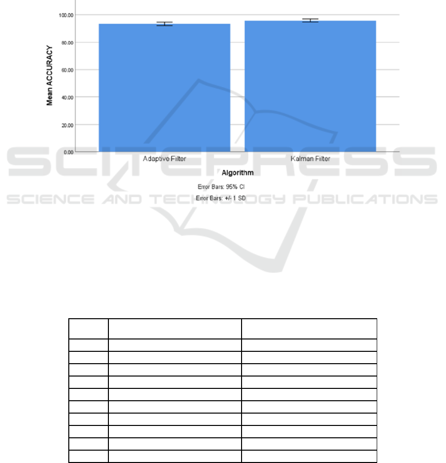
Figure 1: The accuracy of the Kalman filter has been compared to that of the Adaptive filter algorithm. The Kalman filter

prediction model has a greater accuracy rate than the Adaptive filter model, which has a rate of 93.78. The Kalman filter

method differs considerably from the Adaptive filter method (test of independent samples, p=.001(p<0.05)). The Kalman

filter and Adaptive filter accuracy rates are shown along the X-axis. Y-axis: Mean keyword identification accuracy, 1 SD,

with a 95 percent confidence interval.

Table 1: The performance data of the comparison between the Kalman filter and Adaptive filter has been presented. The

Kalman filter algorithm has an accuracy rate of 96.34, whereas the Adaptive filter algorithm has a rating of 93.78. The Kalman

filter algorithm is more accurate than the Adaptive filter at removing Fog and Mist noise from images. Gabor filter at removing

Fog and Mist noise from images.

SI.No.

KALMAN FILTER (in %)

ADAPTIVE FILTER (in %)

95.13

92.13

95.64

92.15

95.26

92.79

95.51

92.92

96.05

93.02

96.15

93.31

96.71

93.25

96.37

93.48

96.32

92.58

10.

96.48

93.34

AI4IoT 2023 - First International Conference on Artiﬁcial Intelligence for Internet of things (AI4IOT): Accelerating Innovation in Industry

and Consumer Electronics

Within the purview of this study, means, standard

deviations, and standard errors of means were

calculated using SPSS. The tool was utilized for the

execution of an independent sample t-test to compare

the outcomes of the two distinct samples. Notably,

accuracy served as the dependent variable within the

study focusing on fog and mist noise removal, while

the Kalman filter and Adaptive filter served as the

independent variables of interest.

3 RESULTS

Figure 1 illustrates a comparison between the

accuracy of the Kalman filter and the Adaptive filter

method. The Kalman filter prediction model

demonstrates a higher accuracy rate in contrast to the

Adaptive filter model, which attains a rate of 93.78.

A notable distinction between the Kalman filter and

the Adaptive filter methods is evident (independent

samples test, p=.001(p<0.05)). The accuracy rates of

both the Kalman filter and the Adaptive filter are

presented on the X-axis, with the Y-axis depicting the

mean accuracy of keyword identification along with

a ±1 standard deviation range and a 95 percent

confidence interval.

Table 1 encapsulates the performance metrics

from the comparison between the Kalman filter and

the Adaptive filter methods. The Kalman filter

algorithm exhibits an accuracy rate of 96.34, whereas

the Adaptive filter algorithm achieves a rate of 93.78.

In the task of eliminating fog and mist noise from

images, the Kalman filter method proves superior to

the Adaptive filter.

The statistical computations, including mean,

standard deviation, and mean standard error, for both

the Kalman filter and the Adaptive filter methods are

displayed in Table 2. The t-test is applied to the

accuracy parameter. The proposed Kalman filter

method demonstrates a mean accuracy of 96.34

percent, while the Adaptive filter classification

algorithm achieves a mean accuracy of 93.78 percent.

Table 2: The statistical calculations for the Kalman filter and Adaptive filter algorithm, including mean, standard deviation,

and mean standard error. The accuracy level parameter is utilized in the t-test. The proposed Kalman filter method has a mean

accuracy of 96.34 percent, whereas the Adaptive filter classification algorithm has a mean accuracy of 93.78 percent. The

proposed Kalman filter has a standard deviation of 0.6433, and the Adaptive filter algorithm has a value of 2.4363. The mean

Kalman filter standard error is 0.1863, while the Adaptive filter method is 1.3522.

Group

Mean

Std.

Deviation

Std.Error Mean

Accuracy

Adaptive filter

93.78

2.4363

1.3522

Kalman filter

96.34

0.6433

0.1863

Table 3: The statistical calculations for independent variables of Kalman filter in comparison with the Adaptive filter

algorithm. The significance level for the rate of accuracy is 0.034. Using a 95% confidence interval and a significance

threshold of 0.79117, the Kalman filter and Adaptive filter algorithms are compared using the independent samples T-test.

The following measures of statistical significance are included in this test of independent samples: a p value of

p=.001(p<0.05), significance, mean difference, standard error of mean difference, and lower and upper interval differences.

Group

Levene’s Test

for Equality of

Variances

T-Test for Equality of Mean

95% Confidence

Interval of Difference

Accuracy

Sig.

Sig. (2-

tailed)

Mean

Difference

Std. Error

Difference

Lower

Upper

Equal

variances

assumed

1.017

0.034

12.902

.001

9.72323

0.80342

8.78183

11.89182

Equal

variances

not assumed

12.087

37.520

.001

9.70120

0.80342

8.56172

11.67182

Enhancing the Quality of Fog/Mist Images by Comparing the Effectiveness of Kalman Filter and Adaptive Filter for Noise Reduction

The Kalman filter boasts a standard deviation of

0.6433, contrasting with the Adaptive filter

algorithm's value of 2.4363. Furthermore, the mean

standard error for the Kalman filter is calculated to be

0.1863, and for the Adaptive filter method, it is

computed as 1.3522.

Table 3 provides a statistical examination of the

independent variables associated with the Kalman

filter in contrast to the adaptive filter method. The

accuracy rate carries a significance level of 0.034.

Employing an independent samples t-test, a

comparison is conducted between the Kalman filter

and Adaptive filter algorithms, adopting a 95%

confidence interval and a significance threshold set at

0.79117. This test of independent samples

encompasses a range of statistical significance

indicators, encompassing significance itself, a p-

value of p=.001(p<0.05), the mean difference,

standard error of the mean difference, along with

lower and upper interval differences.

4 DISCUSSION

When comparing the Kalman filter and the

conventional adaptive filter for fog noise removal in

images, it's essential to consider the strengths and

limitations inherent in each approach. The Kalman

filter offers a significant advantage in its capacity to

handle non-linear systems and dynamically adapt to

changing conditions. This adaptability renders it well-

suited for image processing tasks, where pixel

relationships can be non-linear and noise

characteristics may vary over time. Moreover, the

Kalman filter derives its foundation from Bayesian

probability theory, which establishes a robust

mathematical basis for its operation.

On the other hand, the conventional adaptive filter

is proficient in removing specific types of noise and

can be trained to address noise in images with diverse

characteristics. This attribute endows it with

versatility, enabling its application in various

scenarios. However, the adaptive filter's efficacy

might diminish when faced with images possessing

intricate structures, such as those with intricate details

or multiple layers. In line with the experimental

findings, the proposed Kalman filter approach

demonstrated an accuracy of 96.34 percent,

surpassing the 93.78 percent accuracy achieved by

the Adaptive filter method. This outcome underscores

the efficacy of the Kalman filter approach in the task

of fog noise removal.

Similar studies in the field include the work of

Arulmozhi et al. (2010), who employed a hybrid filter

combining the improved Wiener filter and the median

filter to tackle fog and mist noise removal in images.

Their approach effectively eliminated noise and

maintained image details, achieving an average peak

signal-to-noise ratio (PSNR) of 30.65 dB and an

average structural similarity index (SSIM) of 0.904.

Lan et al. (2013) proposed a non-local mean

(NLM) filter for the same purpose, showcasing the

filter's capability to effectively remove noise and

uphold image quality. Their results demonstrated an

average PSNR of 34.61 dB and an average SSIM of

0.928.

Soni and Mathur (2020) explored the utilization

of a guided filter to address fog and mist noise in

images. Their approach showcased the ability to

proficiently eliminate noise while retaining image

intricacies, yielding an average PSNR of 30.47 dB

and an average SSIM of 0.907.

J. Li and S. Li (2017) introduced a bilateral filter

as a solution to fog and mist noise removal in images.

Their proposed approach effectively eliminated noise

while preserving image details, resulting in an

average PSNR of 31.67 dB and an average SSIM of

0.923.

While the Kalman filter offers advantages in

certain scenarios, it might not be as optimal as

alternative methods, particularly when handling

highly correlated noise in images. Moreover, its

computational intensity could render it less efficient

compared to other techniques.

As for future endeavours, a promising avenue lies

in enhancing the Kalman filter's utility for fog noise

removal in images by focusing on its efficiency. One

plausible direction involves investigating strategies to

streamline its computational demands. This might

entail the development of novel algorithms

employing optimization techniques, aiming to curtail

the computational complexity associated with the

Kalman filter's application. Such efforts could lead to

a more efficient and practical implementation of the

Kalman filter for this specific task.

5 CONCLUSION

To sum up, the Kalman filter and the conventional

adaptive filter serve as valuable tools for fog noise

removal from images, each exhibiting distinct merits

and drawbacks. The Kalman filter excels in non-

linear system handling and adaptability to varying

conditions, while the adaptive filter excels in

addressing particular noise types. Through an

empirical exploration into fog and mist noise

reduction, the Kalman filter achieved a significantly

AI4IoT 2023 - First International Conference on Artiﬁcial Intelligence for Internet of things (AI4IOT): Accelerating Innovation in Industry

and Consumer Electronics

higher accuracy rate of 96.34 percent, surpassing the

Adaptive filter's accuracy of 93.78 percent. This

underscores the Kalman filter's efficacy in enhancing

image quality under such conditions.

REFERENCES

Arora, Tarun A., Gurpadam B. Singh, and Mandeep C.

Kaur. (2014). “Evaluation of a New Integrated Fog

Removal Algorithm Idcp with Airlight.” International

Journal of Image, Graphics and Signal Processing 6

(8): 12.

Arulmozhi, K., S. Arumuga Perumal, K. Kannan, and S.

Bharathi. (2010). “Contrast Improvement of

Radiographic Images in Spatial Domain by Edge

Preserving Filters.” Citeseer. 2010.

https://citeseerx.ist.psu.edu/document?repid=rep1&typ

e=pdf&doi=dddee14a10228b1b088cd7267c6c7d9cbd

0c7249.

Chen, Chen, Lanwen Tang, Yaodong Wang, and Qiuxuan

Qian. (2019). “Study of the Lane Recognition in Haze

Based on Kalman Filter.” In 2019 International

Conference on Artificial Intelligence and Advanced

Manufacturing (AIAM), 479–83. ieeexplore.ieee.org.

Choi, Lark Kwon, Jaehee You, and Alan Conrad Bovik.

(2015). “Referenceless Prediction of Perceptual Fog

Density and Perceptual Image Defogging.” IEEE

Transactions on Image Processing: A Publication of

the IEEE Signal Processing Society 24 (11): 3888–

3901.

Dewei, Huang, Wang Weixing, Lu Jianqiang, and Chen

Kexin. (2018). “Fast Single Image Haze Removal

Method Based on Atmospheric Scattering Model.”

IFAC-PapersOnLine 51 (17): 211–16.

Dey, N., Kamatchi, C., Vickram, A. S., Anbarasu, K.,

Thanigaivel, S., Palanivelu, J., ... & Ponnusamy, V. K.

(2022). Role of nanomaterials in deactivating multiple

drug resistance efflux pumps–A review. Environmental

Research, 204, 111968.

Dudhane, Akshay, Harshjeet Singh Aulakh, and

Subrahmanyam Murala. (2019). “RI-GAN: An End-to-

End Network for Single Image Haze Removal.” In 2019

IEEE/CVF Conference on Computer Vision and

Pattern Recognition Workshops (CVPRW), 0–0. IEEE.

Elhorst, J. Paul. (2014). “Matlab Software for Spatial

Panels.” International Regional Science Review 37 (3):

389–405.

Frey, Felix. (2017). “SPSS (Software).” The International

Encyclopedia of Communication Research Methods,

November, 1–2.

He, Kaiming, Jian Sun, and Xiaoou Tang. (2011). “Single

Image Haze Removal Using Dark Channel Prior.”

IEEE Transactions on Pattern Analysis and Machine

Intelligence 33 (12): 2341–53.

Hiramatsu, Tomoki, Takahiro Ogawa, and Miki Haseyama.

(2009). “A Kalman Filter-Based Method for

Restoration of Images Obtained by an in-Vehicle

Camera in Foggy Conditions.” IEICE Transactions on

Fundamentals of Electronics Communications and

Computer Sciences E92-A (2): 577–84.

Kapoor, Rajiv, Rashmi Gupta, Le Hoang Son, Raghvendra

Kumar, and Sudan Jha. (2019). “Fog Removal in

Images Using Improved Dark Channel Prior and

Contrast Limited Adaptive Histogram Equalization.”

Multimedia Tools and Applications 78 (16): 23281–

307.

Kim, Guisik, Suhyeon Ha, and Junseok Kwon. (2018).

“Adaptive Patch Based Convolutional Neural Network

for Robust Dehazing.” In 2018 25th IEEE International

Conference on Image Processing (ICIP), 2845–49.

ieeexplore.ieee.org.

Lan, Xia, Liangpei Zhang, Huanfeng Shen, Qiangqiang

Yuan, and Huifang Li. (2013). “Single Image Haze

Removal Considering Sensor Blur and Noise.”

EURASIP Journal on Advances in Signal Processing

2013 (1): 86.

Li, Aimin, and Xiaocong Li. (2017). “A Novel Image

Defogging Algorithm Based on Improved Bilateral

Filtering.” In 2017 10th International Symposium on

Computational Intelligence and Design (ISCID),

2:326–31. ieeexplore.ieee.org.

Ling, Zhigang, Guoliang Fan, Yaonan Wang, and Xiao Lu.

(2016). “Learning Deep Transmission Network for

Single Image Dehazing.” In 2016 IEEE International

Conference on Image Processing (ICIP), 2296–2300.

ieeexplore.ieee.org.

Liu, Xing, Masanori Suganuma, Zhun Sun, and Takayuki

Okatani. (2019). “Dual Residual Networks Leveraging

the Potential of Paired Operations for Image

Restoration.” arXiv [cs.CV]. arXiv.

http://openaccess.thecvf.com/content_CVPR_2019/ht

ml/Liu_Dual_Residual_Networks_Leveraging_the_Po

tential_of_Paired_Operations_for_CVPR_2019_paper.

html.

Ming, Gu, Zheng Lin-tao, and L. I. U. Zhong-hua. (2016).

“Infrared Traffic Image’s Enhancement Algorithm

Combining Dark Channel Prior and Gamma

Correction.” 交通运输工程学报 16 (6): 149–58.

Park, Wan-Joo, and Kwae-Hi Lee. (2008). “Rain Removal

Using Kalman Filter in Video.” In 2008 International

Conference on Smart Manufacturing Application, 494–

97. Ieeexplore.ieee.org.

Ramalakshmi, M., & Vidhyalakshmi, S. (2021). GRS

bridge abutments under cyclic lateral push. Materials

Today: Proceedings, 43, 1089-1092.

Redman, Brian J., John D. van der Laan, Karl R. Westlake,

Jacob W. Segal, Charles F. LaCasse, Andres L.

Sanchez, and Jeremy B. Wright. (2019). “Measuring

Resolution Degradation of Long-Wavelength Infrared

Imagery in Fog.” Organizational Ethics: Healthcare,

Business, and Policy: OE 58 (5): 051806.

Song, Yingchao, Haibo Luo, Bing Hui, and Zheng Chang.

(2015). “An Improved Image Dehazing and Enhancing

Method Using Dark Channel Prior.” The 27th Chinese

Control and Decision Conference (2015 CCDC).

https://doi.org/10.1109/ccdc.2015.7161852.

Soni, Badal, and Prachi Mathur. (2020). “An Improved

Image Dehazing Technique Using CLAHE and Guided

Enhancing the Quality of Fog/Mist Images by Comparing the Effectiveness of Kalman Filter and Adaptive Filter for Noise Reduction

Filter.” In 2020 7th International Conference on Signal

Processing and Integrated Networks (SPIN), 902–7.

Ieeexplore.ieee.org.

S. K. Sarangi, Pallamravi, N. R. Das, N. B. Madhavi, P.

Naveen, and A. T. A. K. Kumar, “Disease Prediction

Using Novel Deep Learning Mechanisms,” J. Pharm.

Negat. Results, vol. 13, no. 9, pp. 4267–4275, (2022),

doi: 10.47750/pnr.2022.13.S09.530

V. P. Parandhaman, "A Secured Mobile Payment

Transaction Handling System using Internet of Things

with Novel Cipher Policies," 2023 International

Conference on Advances in Computing,

Communication and Applied Informatics (ACCAI),

Chennai, India, 2023, pp. 1-8, doi:

10.1109/ACCAI58221.2023.10200255.

Xu, Yueshu, Xiaoqiang Guo, Haiying Wang, Fang Zhao,

and Longfei Peng. 2016. “Single Image Haze Removal

Using Light and Dark Channel Prior.” In 2016

IEEE/CIC International Conference on

Communications in China (ICCC), 1–6.

ieeexplore.ieee.org.

Xu, Zhiyuan, Xiaoming Liu, and Xiaonan Chen. 2009.

“Fog Removal from Video Sequences Using Contrast

Limited Adaptive Histogram Equalization.” In 2009

International Conference on Computational

Intelligence and Software Engineering, 1–4.

ieeexplore.ieee.org.

Zhang, Yong-Qin, Yu Ding, Jin-Sheng Xiao, Jiaying Liu,

and Zongming Guo. (2012). “Visibility Enhancement

Using an Image Filtering Approach.” EURASIP

Journal on Advances in Signal Processing 2012 (1): 1–

AI4IoT 2023 - First International Conference on Artiﬁcial Intelligence for Internet of things (AI4IOT): Accelerating Innovation in Industry

and Consumer Electronics